Tag Archives: quantitative research

Scientific Measurement

When it comes to measurement in research. There are some rules and concepts a student needs to be aware of that are not difficult to master but can be tricky. Measurement can be conducted at different levels. The two main levels are categorical and continuous.

Categorical measurement involves counting discrete values. An example of something measured at the categorical level is the cellphone brand. A cellphone can be Apple or Samsung, but it cannot be both. In other words, there is no phone out there that is half Samsung and half Apple. Being an Apple or Samsung phone is mutually exclusive, and no phone can have both qualities simultaneously. Therefore, categorical measurement deals with whole numbers, and generally, there are no additional rules to keep in mind.

However, with continuous measurement, things become more complicated. Continuous measurement involves an infinite number of potential values. For example, distance and weight can be measured continuously. A distance can be 1 km or 1.24 km, or 1.234. It all depends on the precision of the measurement tool. The point to remember now is that categorical measurement often has limit values that can be used while continuous has an almost limitless set of values that can be used.

Since the continuous measurement is so limitless, there are several additional concepts that a student needs to mastery. One, the units involved must always be included. At least one reason for this is that it is common to convert units from one to the other. However, with categorical data, you generally will not convert phone units to some other unit.

A second concern is to be aware of the precision and accuracy of your measurement. Precision has to do with how fine the measurement is. For example, you can measure something the to the tenth, the hundredth, the thousandth, etc. As you add decimals, you are improving the precision. Accuracy is how correct the measurement is. If a person’s weight is 80kg, but your measurement is 63.456789kg, this is an example of high precision with low accuracy.

Another important concept when dealing with continuous measurement is understanding how many significant figures are involved. The ideas of significant figures are explored below.

Significant figures

Significant figures are digit that contributes to the precision of a measurement. This term is not related to significance as defined in statistics related to hypothesis testing.

An example of significant figures is as follows. If you have a scale that measures to the thousandth of a kg, you must report measurements to the thousandths of a kg. For example, 2 kg is not how you would report this based on the precision of your tool. Rather, you would report 2.000kg. This implies that the weight is somewhere between 1.995 and 2.004 kg. This is really important if you are conducting measurements in the scientific domain.

There are also several rules in regards to determining the number of significant figures, and they are explained below

All non zeros are significant
1. Example-123 are all non-zeros and thus are all significant in this case
A zero is significant if it is between two significant numbers
1. example-1023. The 0 is in between 1 and 2 and is thus significant
Zeros are significant if it is at the end of a number and to the right of the decimal
1. Example 2.00: Here, the 0’s are to the right of the decimal, which makes them significant

Each of the examples discussed so far has been individual examples. However, what happens when numbers are added or multiplied. The next section covers this in detail

Significant Figures in Math

Addition/Subtraction

When adding and subtracting measurements, you must report the measurement results with the less precise measurement.

example
115kg – 16.234kg = 98.766kg, but the least precise measurement is 115kg, so we round the answer to 99 kg. This is because our precision is limited to one’s place.

Multiply/Divide

When multiply or dividing measurements report results with the same number of significant figures as the measurement with the fewest significant figures

example 1
16.423 m / 101 m = 0.16260396 m

This number is too long. The second number, 101, has three significant figures, so our answer will have 3 significant figures, 0.163m. The zero to the left of the decimal is insignificant and does not count in the total.

example 2
8.0 cm * 3.208 = 25.664 cm2 or 26cm2 the first number has two significant digits, so the answer can only have two significant figures, which leads to an answer of 26cm2.

Converting Units

Finally, there are rules for converting units as well. To convert units, you must know the relationship that the two units have. For example, there are 2.54 cms per inch. Often this information is provided for you, and simply apply it. Once the relationship between units is known, it is common to use the factor label method for conversion. Below is an example.

To solve this problem, it is simply a matter of canceling the numerator of one fraction and the denominator of another fraction because, in this example, they are the same. This is shown below.

Essentially there was no calculation involved. Understanding shortcuts like this saves a tremendous amount of time. What is really important is that this idea applies to units as well. Below is an example.

In the example above, we are converting inches to meters. We know that there is 2.54cm in 1 inch. We set up our fractions as shown above. The inches cancel because they are in the numerator of one fraction and the denominator of another. The only unit left is cm. We multiply across and get our answer. Since 24.0cm has the fewest number of significant figures are the answer will also have three significant figures, and that is why its 61.0cm

Scientiifc Nottation

There can be problems with following the rules of significant figures. For example, if you want to convert meters to centimeters. There can be a problem.

The answer should only have three significant figures, but our answer has one significant figure. We need to move two zeros to the right of the decimal.

This is done with scientific notation as shown vbelow.

This simple trick allows us to keep the number of signifcant figures that we need without hhanging the value of then umber.

Below is an example of how to do this with a really small number that is a decimal.

Conclusion

This post explains some of the rules involved with numbers in scientific measurement. These rules are critical in terms of meeting expectations for communicating quantitative results.

Understanding Variables

Leave a reply

In research, there are many terms that have the same underlying meaning which can be confusing for researchers as they try to complete a project. The problem is that people have different backgrounds and learn different terms during their studies and when they try to work with others there is often confusion over what is what.

In this post, we will try to clarify as much as possible various terms that are used when referring to variables. We will look at the following during this discussion

Definition of a variable
Minimum knowledge of the characteristics of a variable in research
Various synonyms of variable

Definition

The word variable has the root of “vary” and the suffix “able”. This literally means that a variable is something that is able to change. Examples include such concepts as height, weigh, salary, etc. All of these concepts change as you gather data from different people. Statistics is primarily about trying to explain and or understand the variability of variables.

However, to make things more confusing there are times in research when a variable dies not change or remains constant. This will be explained in greater detail in a moment.

Minimum You Need to Know

Two broad concepts that you need to understand regardless of the specific variable terms you encounter are the following

Whether the variable(s) are independent or dependent
Whether the variable(s) are categorical or continuous

When we speak of independent and dependent variables we are looking at the relationship(s) between variables. Dependent variables are explained by independent variables. Therefore, one dimension of variables is understanding how they relate to each other and the most basic way to see this is independent vs dependent.

The second dimension to consider when thinking about variables is how they are measured which is captured with the terms categorical or continuous. A categorical variable has a finite number of values that can be used. Examples in clue gender, hair color, or cellphone brand. A person can only be male or female, have blue or brown eyes, and can only have one brand of cellphone.

Continuous variables are variables that can take on an infinite number of values. Salary, temperature, etc are all continuous in nature. It is possible to limit a continuous variable to categorical variable by creating intervals in which to place values. This is commonly done when creating bins for histograms. In sum, here are the four possible general variable types below

Independent categorical
Independent continuous
Dependent categorical
Dependent continuous

Natural, most models have one dependent categorical or continuous variable, however you can have any combination of continuous and categorical variables as independents. Remember that all variables have the above characteristics despite whatever terms is used for them.

Variable Synonyms

Below is a list of various names that variables go by in different disciplines. This is by no means an exhaustive list.

Experimental variable

A variable whose values are independent of any changes in the values of other variables. In other words, an experimental variable is just another term for independent variable.

Manipulated Variable

A variable that is independent in an experiment but whose value/behavior the researcher is able to control or manipulate. This is also another term for an independent variable.

Control Variable

A variable whose value does not change. Controlling a variable helps to explain the relationship between the independent and dependent variable in an experiment by making sure the control variable has not influenced in the model

Responding Variable

The dependent variable in an experiment. It responds to the experimental variable.

Intervening Variable

This is a hypothetical variable. It is used to explain the causal links between variables. Since they are hypothetical, they are observed in an actual experiment. For example, if you are looking at a strong relationship between income and life expectancy and find a positive relationship. The intervening variable for this may be access to healthcare. People who make more money have more access to health care and this contributes to them often living longer.

Mediating Variable

This is the same thing as an intervening variable. The difference being often that the mediating variable is not always hypothetical in nature and is often measured it’s self.

Confounding Variable

A confounder is a variable that influences both the independent and dependent variable, causing a spurious or false association. Often a confounding variable is a causal idea and cannot be described in terms of correlations or associations with other variables. In other words, it is often the same thing as an intervening variable.

Explanatory Variable

This variable is the same as an independent variable. The difference being that an independent variable is not influenced by any other variables. However, when independence is not for sure, than the variable is called an explanatory variable.

Predictor Variable

A predictor variable is an independent variable. This term is commonly used for regression analysis.

Outcome Variable

An outcome variable is a dependent variable in the context of regression analysis.

Observed Variable

This is a variable that is measured directly. An example would be gender or height. There is no psychology construct to infer the meaning of such variables.

Unobserved Variable

Unobserved variables are constructs that cannot be measured directly. In such situations, observe variables are used to try to determine the characteristic of the unobserved variable. For example, it is hard to measure addiction directly. Instead, other things will be measure to infer addiction such as health, drug use, performance, etc. The measures of this observed variables will indicate the level of the unobserved variable of addiction

Features

A feature is an independent variable in the context of machine learning and data science.

Target Variable

A target variable is the dependent variable in the context f machine learning and data science.

To conclude this, below is a summary of the different variables discussed and whether they are independent, dependent, or neither.

Independent	Dependent	Neither
Experimental	Responding	Control
Manipulated	Target	Explanatory
Predictor	Outcome	Intervening
Feature		Mediating
		Observed
		Unobserved
		Confounding

You can see how confusing this can be. Even though variables are mostly independent or dependent, there is a class of variables that do not fall into either category. However, for most purposes, the first to columns cover the majority of needs in simple research.

Conclusion

The confusion over variables is mainly due to an inconsistency in terms across variables. There is nothing right or wrong about the different terms. They all developed in different places to address the same common problem. However, for students or those new to research, this can be confusing and this post hopefully helps to clarify this.

Research Questions, Variables, and Statistics

Leave a reply

Working with students over the years has led me to the conclusion that often students do not understand the connection between variables, quantitative research questions and the statistical tools

used to answer these questions. In other words, students will take statistics and pass the class. Then they will take research methods, collect data, and have no idea how to analyze the data even though they have the necessary skills in statistics to succeed.

This means that the students have a theoretical understanding of statistics but struggle in the application of it. In this post, we will look at some of the connections between research questions and statistics.

Variables

Variables are important because how they are measured affects the type of question you can ask and get answers to. Students often have no clue how they will measure a variable and therefore have no idea how they will answer any research questions they may have.

Another aspect that can make this confusing is that many variables can be measured more than one way. Sometimes the variable “salary” can be measured in a continuous manner or in a categorical manner. The superiority of one or the other depends on the goals of the research.

It is critical to support students to have a thorough understanding of variables in order to support their research.

Types of Research Questions

In general, there are two types of research questions. These two types are descriptive and relational questions. Descriptive questions involve the use of descriptive statistic such as the mean, median, mode, skew, kurtosis, etc. The purpose is to describe the sample quantitatively with numbers (ie the average height is 172cm) rather than relying on qualitative descriptions of it (ie the people are tall).

Below are several example research questions that are descriptive in nature.

What is the average height of the participants in the study?
What proportion of the sample is passed the exam?
What are the respondents perceptions towards the cafeteria?

These questions are not intellectually sophisticated but they are all answerable with descriptive statistical tools. Question 1 can be answered by calculating the mean. Question 2 can be answered by determining how many passed the exam and dividing by the total sample size. Question 3 can be answered by calculating the mean of all the survey items that are used to measure respondents perception of the cafeteria.

Understanding the link between research question and statistical tool is critical. However, many people seem to miss the connection between the type of question and the tools to use.

Relational questions look for the connection or link between variables. Within this type there are two sub-types. Comparison question involve comparing groups. The other sub-type is called relational or an association question.

Comparison questions involve comparing groups on a continuous variable. For example, comparing men and women by height. What you want to know is whether there is a difference in the height of men and women. The comparison here is trying to determine if gender is related to height. Therefore, it is looking for a relationship just not in the way that many student understand. Common comparison questions include the following.male

Is there a difference in height by gender among the participants?
Is there a difference in reading scores by grade level?
Is there a difference in job satisfaction in based on major?

Each of these questions can be answered using ANOVA or if we want to get technical and there are only two groups (ie gender) we can use t-test. This is a broad overview and does not include the complexities of one-sample test and or paired t-test.

Relational or association question involve continuous variables primarily. The goal is to see how variables move together. For example, you may look for the relationship between height and weight of students. Common questions include the following.

Is there a relationship between height and weight?
Does height and show size explain weight?

Questions 1 can be answered by calculating the correlation. Question 2 requires the use of linear regression in order to answer the question.

Conclusion

The challenging as a teacher is showing the students the connection between statistics and research questions from the real world. It takes time for students to see how the question inspire the type of statistical tool to use. Understanding this is critical because it helps to frame the possibilities of what to do in research based on the statistical knowledge one has.

Statistical Learning

1 Reply

Statistical learning is a discipline that focuses on understanding data. Understanding data can happen through classifying or making a numeric prediction which is called supervised learning or finding patterns in data which is called unsupervised learning,

In this post, we will examine the following

History of statistical learning
The purpose of statistical learning
Statistical learning vs Machine learning

History Of Statistical Learning

The early pioneers of statistical learning focused exclusively on supervised learning. Linear regression was developed in the 19th century by Legendre and Gauss. In the 1930’s, Fisher created linear discriminant analysis. Logistic regression was created in the 1940’s as an alternative the linear discriminant analysis.

The developments of the late 19th century to the mid 20th century were limited due to the lack of computational power. However, by the 1970’s things began to change and new algorithms emerged, specifically ones that can handle non-linear relationships

In the 1980’s Friedman and Stone developed classification and regression trees. The term generalized additive models were first used by Hastie and Tibshirani for non-linear generalized models.

Purpose of Statistical Learning

The primary goal of statistical learning is to develop a model of data you currently have to make decisions about the future. In terms of supervised learning with a numeric dependent variable, a teacher may have data on their students and want to predict future academic performance. For a categorical variable, a doctor may use data he has to predict whether someone has cancer or not. In both situations, the goal is to use what one knows to predict what one does not know.

A unique characteristic of supervised learning is that the purpose can be to predict future values or to explain the relationship between the dependent variable and another independent variable(s). Generally, data science is much more focused on prediction while the social sciences seem more concerned with explanations.

For unsupervised learning, there is no dependent variable. In terms of a practical example, a company may want to use the data they have to determine several unique categories of customers they have. Understanding large groups of customer behavior can allow the company to adjust their marketing strategy to cater to the different needs of their vast clientele.

Statistical Learning vs Machine Learning

The difference between statistical learning and machine learning is so small that for the average person it makes little difference. Generally, although some may disagree, these two terms mean essentially the same thing. Often statisticians speak of statistical learning while computer scientist speak of machine learning

Machine learning is the more popular term as it is easier to conceive of a machine learning rather than statistics learning.

Conclusion

Statistical or machine learning is a major force in the world today. With some much data and so much computing power, the possibilities are endless in terms of what kind of beneficial information can be gleaned. However, all this began with people creating a simple linear model in the 19th century.

Ridge Regression in R

Leave a reply

In this post, we will conduct an analysis using ridge regression. Ridge regression is a type of regularized regression. By applying a shrinkage penalty, we are able to reduce the coefficients of many variables almost to zero while still retaining them in the model. This allows us to develop models that have many more variables in them compared to models using the best subset or stepwise regression.

In the example used in this post, we will use the “SAheart” dataset from the “ElemStatLearn” package. We want to predict systolic blood pressure (sbp) using all of the other variables available as predictors. Below is some initial code that we need to begin.

library(ElemStatLearn);library(car);library(corrplot)
library(leaps);library(glmnet);library(caret)

data(SAheart)
str(SAheart)

## 'data.frame':    462 obs. of  10 variables:
##  $ sbp      : int  160 144 118 170 134 132 142 114 114 132 ...
##  $ tobacco  : num  12 0.01 0.08 7.5 13.6 6.2 4.05 4.08 0 0 ...
##  $ ldl      : num  5.73 4.41 3.48 6.41 3.5 6.47 3.38 4.59 3.83 5.8 ...
##  $ adiposity: num  23.1 28.6 32.3 38 27.8 ...
##  $ famhist  : Factor w/ 2 levels "Absent","Present": 2 1 2 2 2 2 1 2 2 2 ...
##  $ typea    : int  49 55 52 51 60 62 59 62 49 69 ...
##  $ obesity  : num  25.3 28.9 29.1 32 26 ...
##  $ alcohol  : num  97.2 2.06 3.81 24.26 57.34 ...
##  $ age      : int  52 63 46 58 49 45 38 58 29 53 ...
##  $ chd      : int  1 1 0 1 1 0 0 1 0 1 ...

A look at the object using the “str” function indicates that one variable “famhist” is a factor variable. The “glmnet” function that does the ridge regression analysis cannot handle factors so we need to convert this to a dummy variable. However, there are two things we need to do before this. First, we need to check the correlations to make sure there are no major issues with multicollinearity Second, we need to create our training and testing data sets. Below is the code for the correlation plot.

p.cor<-cor(SAheart[,-5])
corrplot.mixed(p.cor)

First we created a variable called “p.cor” the -5 in brackets means we removed the 5th column from the “SAheart” data set which is the factor variable “Famhist”. The correlation plot indicates that there is one strong relationship between adiposity and obesity. However, one common cut-off for collinearity is 0.8 and this value is 0.72 which is not a problem.

We will now create are training and testing sets and convert “famhist” to a dummy variable.

ind<-sample(2,nrow(SAheart),replace=T,prob = c(0.7,0.3))
train<-SAheart[ind==1,]
test<-SAheart[ind==2,]
train$famhist<-model.matrix( ~ famhist - 1, data=train ) #convert to dummy variable 
test$famhist<-model.matrix( ~ famhist - 1, data=test )

We are still not done preparing our data yet. “glmnet” cannot use data frames, instead, it can only use matrices. Therefore, we now need to convert our data frames to matrices. We have to create two matrices, one with all of the predictor variables and a second with the outcome variable of blood pressure. Below is the code

predictor_variables<-as.matrix(train[,2:10])
blood_pressure<-as.matrix(train$sbp)

We are now ready to create our model. We use the “glmnet” function and insert our two matrices. The family is set to Gaussian because “blood pressure” is a continuous variable. Alpha is set to 0 as this indicates ridge regression. Below is the code

ridge<-glmnet(predictor_variables,blood_pressure,family = 'gaussian',alpha = 0)

Now we need to look at the results using the “print” function. This function prints a lot of information as explained below.

Df = number of variables including in the model (this is always the same number in a ridge model)
%Dev = Percent of deviance explained. The higher the better
Lambda = The lambda used to attain the %Dev

When you use the “print” function for a ridge model it will print up to 100 different models. Fewer models are possible if the percent of deviance stops improving. 100 is the default stopping point. In the code below we have the “print” function. However, I have only printed the first 5 and last 5 models in order to save space.

print(ridge)

## 
## Call:  glmnet(x = predictor_variables, y = blood_pressure, family = "gaussian",      alpha = 0) 
## 
##        Df      %Dev    Lambda
##   [1,] 10 7.622e-37 7716.0000
##   [2,] 10 2.135e-03 7030.0000
##   [3,] 10 2.341e-03 6406.0000
##   [4,] 10 2.566e-03 5837.0000
##   [5,] 10 2.812e-03 5318.0000
................................
##  [95,] 10 1.690e-01    1.2290
##  [96,] 10 1.691e-01    1.1190
##  [97,] 10 1.692e-01    1.0200
##  [98,] 10 1.693e-01    0.9293
##  [99,] 10 1.693e-01    0.8468
## [100,] 10 1.694e-01    0.7716

The results from the “print” function are useful in setting the lambda for the “test” dataset. Based on the results we can set the lambda at 0.83 because this explains the highest amount of deviance at .20.

The plot below shows us lambda on the x-axis and the coefficients of the predictor variables on the y-axis. The numbers refer to the actual coefficient of a particular variable. Inside the plot, each number corresponds to a variable going from left to right in a data-frame/matrix using the “View” function. For example, 1 in the plot refers to “tobacco” 2 refers to “ldl” etc. Across the top of the plot is the number of variables used in the model. Remember this number never changes when doing ridge regression.

plot(ridge,xvar="lambda",label=T)

As you can see, as lambda increase the coefficient decrease in value. This is how ridge regression works yet no coefficient ever goes to absolute 0.

You can also look at the coefficient values at a specific lambda value. The values are unstandardized but they provide a useful insight when determining final model selection. In the code below the lambda is set to .83 and we use the “coef” function to do this

ridge.coef<-coef(ridge,s=.83,exact = T)
ridge.coef

## 11 x 1 sparse Matrix of class "dgCMatrix"
##                                   1
## (Intercept)            105.69379942
## tobacco                 -0.25990747
## ldl                     -0.13075557
## adiposity                0.29515034
## famhist.famhistAbsent    0.42532887
## famhist.famhistPresent  -0.40000846
## typea                   -0.01799031
## obesity                  0.29899976
## alcohol                  0.03648850
## age                      0.43555450
## chd                     -0.26539180

The second plot shows us the deviance explained on the x-axis and the coefficients of the predictor variables on the y-axis. Below is the code

plot(ridge,xvar='dev',label=T)

The two plots are completely opposite to each other. Increasing lambda cause a decrease in the coefficients while increasing the fraction of deviance explained leads to an increase in the coefficient. You can also see this when we used the “print” function. As lambda became smaller there was an increase in the deviance explained.

We now can begin testing our model on the test data set. We need to convert the test dataset to a matrix and then we will use the predict function while setting our lambda to .83 (remember a lambda of .83 explained the most of the deviance). Lastly, we will plot the results. Below is the code.

test.matrix<-as.matrix(test[,2:10])
ridge.y<-predict(ridge,newx = test.matrix,type = 'response',s=.83)
plot(ridge.y,test$sbp)

The last thing we need to do is calculated the mean squared error. By it’s self this number is useless. However, it provides a benchmark for comparing the current model with any other models you may develop. Below is the code

ridge.resid<-ridge.y-test$sbp
mean(ridge.resid^2)

## [1] 372.4431

Knowing this number, we can develop other models using other methods of analysis to try to reduce it as much as possible.

Linear VS Quadratic Discriminant Analysis in R

Leave a reply

In this post, we will look at linear discriminant analysis (LDA) and quadratic discriminant analysis (QDA). Discriminant analysis is used when the dependent variable is categorical. Another commonly used option is logistic regression but there are differences between logistic regression and discriminant analysis. Both LDA and QDA are used in situations in which there is a clear separation between the classes you want to predict. If the categories are fuzzier logistic regression is often the better choice.

For our example, we will use the “Mathlevel” dataset found in the “Ecdat” package. Our goal will be to predict the sex of a respondent based on SAT math score, major, foreign language proficiency, as well as the number of math, physic, and chemistry classes a respondent took. Below is some initial code to start our analysis.

library(MASS);library(Ecdat)

data("Mathlevel")

The first thing we need to do is clean up the data set. We have to remove any missing data in order to run our model. We will create a dataset called “math” that has the “Mathlevel” dataset but with the “NA”s removed use the “na.omit” function. After this, we need to set our seed for the purpose of reproducibility using the “set.seed” function. Lastly, we will split the data using the “sample” function using a 70/30 split. The training dataset will be called “math.train” and the testing dataset will be called “math.test”. Below is the code

math<-na.omit(Mathlevel)
set.seed(123)
math.ind<-sample(2,nrow(math),replace=T,prob = c(0.7,0.3))
math.train<-math[math.ind==1,]
math.test<-math[math.ind==2,]

Now we will make our model and it is called “lda.math” and it will include all available variables in the “math.train” dataset. Next, we will check the results by calling the model. Finally, we will examine the plot to see how our model is doing. Below is the code.

lda.math<-lda(sex~.,math.train)
lda.math

## Call:
## lda(sex ~ ., data = math.train)
## 
## Prior probabilities of groups:
##      male    female 
## 0.5986079 0.4013921 
## 
## Group means:
##        mathlevel.L mathlevel.Q mathlevel.C mathlevel^4 mathlevel^5
## male   -0.10767593  0.01141838 -0.05854724   0.2070778  0.05032544
## female -0.05571153  0.05360844 -0.08967303   0.2030860 -0.01072169
##        mathlevel^6      sat languageyes  majoreco  majoross   majorns
## male    -0.2214849 632.9457  0.07751938 0.3914729 0.1472868 0.1782946
## female  -0.2226767 613.6416  0.19653179 0.2601156 0.1907514 0.2485549
##          majorhum mathcourse physiccourse chemistcourse
## male   0.05426357   1.441860    0.7441860      1.046512
## female 0.07514451   1.421965    0.6531792      1.040462
## 
## Coefficients of linear discriminants:
##                       LD1
## mathlevel.L    1.38456344
## mathlevel.Q    0.24285832
## mathlevel.C   -0.53326543
## mathlevel^4    0.11292817
## mathlevel^5   -1.24162715
## mathlevel^6   -0.06374548
## sat           -0.01043648
## languageyes    1.50558721
## majoreco      -0.54528930
## majoross       0.61129797
## majorns        0.41574298
## majorhum       0.33469586
## mathcourse    -0.07973960
## physiccourse  -0.53174168
## chemistcourse  0.16124610

plot(lda.math,type='both')

Calling “lda.math” gives us the details of our model. It starts be indicating the prior probabilities of someone being male or female. Next is the means for each variable by sex. The last part is the coefficients of the linear discriminants. Each of these values is used to determine the probability that a particular example is male or female. This is similar to a regression equation.

The plot provides us with densities of the discriminant scores for males and then for females. The output indicates a problem. There is a great deal of overlap between male and females in the model. What this indicates is that there is a lot of misclassification going on as the two groups are not clearly separated. Furthermore, this means that logistic regression is probably a better choice for distinguishing between male and females. However, since this is for demonstrating purposes we will not worry about this.

We will now use the “predict” function on the training set data to see how well our model classifies the respondents by gender. We will then compare the prediction of the model with the actual classification. Below is the code.

math.lda.predict<-predict(lda.math)
math.train$lda<-math.lda.predict$class
table(math.train$lda,math.train$sex)

##         
##          male female
##   male    219    100
##   female   39     73

mean(math.train$lda==math.train$sex)

## [1] 0.6774942

As you can see, we have a lot of misclassification happening. A large amount of false negatives which is a lot of males being classified as female. The overall accuracy is only 59% which is not much better than chance.

We will now conduct the same analysis on the test data set. Below is the code.

lda.math.test<-predict(lda.math,math.test)
math.test$lda<-lda.math.test$class
table(math.test$lda,math.test$sex)

##         
##          male female
##   male     92     43
##   female   23     20

mean(math.test$lda==math.test$sex)

## [1] 0.6292135

As you can see the results are similar. To put it simply, our model is terrible. The main reason is that there is little distinction between males and females as shown in the plot. However, we can see if perhaps a quadratic discriminant analysis will do better

QDA allows for each class in the dependent variable to have its own covariance rather than a shared covariance as in LDA. This allows for quadratic terms in the development of the model. To complete a QDA we need to use the “qda” function from the “MASS” package. Below is the code for the training data set.

math.qda.fit<-qda(sex~.,math.train)
math.qda.predict<-predict(math.qda.fit)
math.train$qda<-math.qda.predict$class
table(math.train$qda,math.train$sex)

##         
##          male female
##   male    215     84
##   female   43     89

mean(math.train$qda==math.train$sex)

## [1] 0.7053364

You can see there is almost no difference. Below is the code for the test data.

math.qda.test<-predict(math.qda.fit,math.test)
math.test$qda<-math.qda.test$class
table(math.test$qda,math.test$sex)

##         
##          male female
##   male     91     43
##   female   24     20

mean(math.test$qda==math.test$sex)

## [1] 0.6235955

Still disappointing. However, in this post, we reviewed linear discriminant analysis as well as learned about the use of quadratic linear discriminant analysis. Both of these statistical tools are used for predicting categorical dependent variables. LDA assumes shared covariance in the dependent variable categories will QDA allows for each category in the dependent variable to have its own variance.

Probability,Odds, and Odds Ratio

Leave a reply

In logistic regression, there are three terms that are used frequently but can be confusing if they are not thoroughly explained. These three terms are probability, odds, and odds ratio. In this post, we will look at these three terms and provide an explanation of them.

Probability

Probability is probably (no pun intended) the easiest of these three terms to understand. Probability is simply the likelihood that a certain event will happen. To calculate the probability in the traditional sense you need to know the number of events and outcomes to find the probability.

Bayesian probability uses prior probabilities to develop a posterior probability based on new evidence. For example, at one point during Super Bowl LI the Atlanta Falcons had a 99.7% chance of winning. This was base don such factors as the number points they were ahead and the time remaining. As these changed, so did the probability of them winning. yet the Patriots still found a way to win with less than a 1% chance

Bayesian probability was also used for predicting who would win the 2016 US presidential race. It is important to remember that probability is an expression of confidence and not a guarantee as we saw in both examples.

Odds

Odds are the expression of relative probabilities. Odds are calculated using the following equation

^{probability of the event}⁄ _{1 – probability of the event}

For example, at one point during Super Bowl LI the odds of the Atlanta Falcons winning were as follows

^0.997⁄ _{1 – 0.997 = 332}

This can be interpreted as the odds being 332 to 1! This means that Atlanta was 332 times more likely to win the Super Bowl then loss the Super Bowl.

Odds are commonly used in gambling and this is probably (again no pun intended) where most of us have heard the term before. The odds is just an extension of probabilities and they are most commonly expressed as a fraction such as one in four, etc.

Odds Ratio

A ratio is the comparison of two numbers and indicates how many times one number is contained or contains another number. For example, a ration of boys to girls is 5 to 1 it means that there are five boys for every one girl.

By extension odds ratio is the comparison of two different odds. For example, if the odds of Team A making the playoffs is 45% and the odds of Team B making the playoffs is 35% the odds ratio is calculated as follows.

^0.45⁄ _{0.35 = 1.28}

Team A is 1.28 more likely to make the playoffs then Team B.

The value of the odds and the odds ratio can sometimes be the same. Below is the odds ratio of the Atlanta Falcons winning and the New Patriots winning Super Bowl LI

^0.997⁄ _{0.003 = 332}

As such there is little difference between odds and odds ratio except that odds ratio is the ratio of two odds ratio. As you can tell, there is a lot of confusion about this for the average person. However, understanding these terms is critical to the application of logistic regression.

Best Subset Regression in R

1 Reply

In this post, we will take a look at best subset regression. Best subset regression fits a model for all possible feature or variable combinations and the decision for the most appropriate model is made by the analyst based on judgment or some statistical criteria.

Best subset regression is an alternative to both Forward and Backward stepwise regression. Forward stepwise selection adds one variable at a time based on the lowest residual sum of squares until no more variables continue to lower the residual sum of squares. Backward stepwise regression starts with all variables in the model and removes variables one at a time. The concern with stepwise methods is they can produce biased regression coefficients, conflicting models, and inaccurate confidence intervals.

Best subset regression bypasses these weaknesses of stepwise models by creating all models possible and then allowing you to assess which variables should be included in your final model. The one drawback to best subset is that a large number of variables means a large number of potential models, which can make it difficult to make a decision among several choices.

In this post, we will use the “Fair” dataset from the “Ecdat” package to predict marital satisfaction based on age, Sex, the presence of children, years married, religiosity, education, occupation, and the number of affairs in the past year. Below is some initial code.

library(leaps);library(Ecdat);library(car);library(lmtest)

data(Fair)

We begin our analysis by building the initial model with all variables in it. Below is the code

fit<-lm(rate~.,Fair)
summary(fit)

## 
## Call:
## lm(formula = rate ~ ., data = Fair)
## 
## Residuals:
##     Min      1Q  Median      3Q     Max 
## -3.2049 -0.6661  0.2298  0.7705  2.2292 
## 
## Coefficients:
##              Estimate Std. Error t value Pr(>|t|)    
## (Intercept)  3.522875   0.358793   9.819  < 2e-16 ***
## sexmale     -0.062281   0.099952  -0.623  0.53346    
## age         -0.009683   0.007548  -1.283  0.20005    
## ym          -0.019978   0.013887  -1.439  0.15079    
## childyes    -0.206976   0.116227  -1.781  0.07546 .  
## religious    0.042142   0.037705   1.118  0.26416    
## education    0.068874   0.021153   3.256  0.00119 ** 
## occupation  -0.015606   0.029602  -0.527  0.59825    
## nbaffairs   -0.078812   0.013286  -5.932 5.09e-09 ***
## ---
## Signif. codes:  0 '***' 0.001 '**' 0.01 '*' 0.05 '.' 0.1 ' ' 1
## 
## Residual standard error: 1.03 on 592 degrees of freedom
## Multiple R-squared:  0.1405, Adjusted R-squared:  0.1289 
## F-statistic:  12.1 on 8 and 592 DF,  p-value: 4.487e-16

The initial results are already interesting even though the r-square is low. When couples have children the have less marital satisfaction than couples without children when controlling for the other factors and this is the strongest regression weight. In addition, the more education a person has there is an increase in marital satisfaction. Lastly, as the number of affairs increases there is also a decrease in marital satisfaction. Keep in mind that the “rate” variable goes from 1 to 5 with one meaning a terrible marriage to five being a great one. The mean marital satisfaction was 3.52 when controlling for the other variables.

We will now create our subset models. Below is the code.

sub.fit<-regsubsets(rate~.,Fair)
best.summary<-summary(sub.fit)

In the code above we create the sub models using the “regsubsets” function from the “leaps” package and saved it in the variable called “sub.fit”. We then saved the summary of “sub.fit” in the variable “best.summary”. We will use the “best.summary” “sub.fit variables several times to determine which model to use.

There are many different ways to assess the model. We will use the following statistical methods that come with the results from the “regsubset” function.

Mallow’ Cp
Bayesian Information Criteria

We will make two charts for each of the criteria above. The plot to the left will explain how many features to include in the model. The plot to the right will tell you which variables to include. It is important to note that for both of these methods, the lower the score the better the model. Below is the code for Mallow’s Cp.

par(mfrow=c(1,2))
plot(best.summary$cp)
plot(sub.fit,scale = "Cp")

The plot on the left suggests that a four feature model is the most appropriate. However, this chart does not tell me which four features. The chart on the right is read in reverse order. The high numbers are at the bottom and the low numbers are at the top when looking at the y-axis. Knowing this, we can conclude that the most appropriate variables to include in the model are age, children presence, education, and number of affairs. Below are the results using the Bayesian Information Criterion

par(mfrow=c(1,2))
plot(best.summary$bic)
plot(sub.fit,scale = "bic")

These results indicate that a three feature model is appropriate. The variables or features are years married, education, and number of affairs. Presence of children was not considered beneficial. Since our original model and Mallow’s Cp indicated that presence of children was significant we will include it for now.

Below is the code for the model based on the subset regression.

fit2<-lm(rate~age+child+education+nbaffairs,Fair)
summary(fit2)

## 
## Call:
## lm(formula = rate ~ age + child + education + nbaffairs, data = Fair)
## 
## Residuals:
##     Min      1Q  Median      3Q     Max 
## -3.2172 -0.7256  0.1675  0.7856  2.2713 
## 
## Coefficients:
##              Estimate Std. Error t value Pr(>|t|)    
## (Intercept)  3.861154   0.307280  12.566  < 2e-16 ***
## age         -0.017440   0.005057  -3.449 0.000603 ***
## childyes    -0.261398   0.103155  -2.534 0.011531 *  
## education    0.058637   0.017697   3.313 0.000978 ***
## nbaffairs   -0.084973   0.012830  -6.623 7.87e-11 ***
## ---
## Signif. codes:  0 '***' 0.001 '**' 0.01 '*' 0.05 '.' 0.1 ' ' 1
## 
## Residual standard error: 1.029 on 596 degrees of freedom
## Multiple R-squared:  0.1352, Adjusted R-squared:  0.1294 
## F-statistic: 23.29 on 4 and 596 DF,  p-value: < 2.2e-16

The results look ok. The older a person is the less satisfied they are with their marriage. If children are present the marriage is less satisfying. The more educated the more satisfied they are. Lastly, the higher the number of affairs indicate less marital satisfaction. However, before we get excited we need to check for collinearity and homoscedasticity. Below is the code

vif(fit2)

##       age     child education nbaffairs 
##  1.249430  1.228733  1.023722  1.014338

No issues with collinearity.For vif values above 5 or 10 indicate a problem. Let’s check for homoscedasticity

par(mfrow=c(2,2))
plot(fit2)

The normal qqplot and residuals vs leverage plot can be used for locating outliers. The residual vs fitted and the scale-location plot do not look good as there appears to be a pattern in the dispersion which indicates homoscedasticity. To confirm this we will use Breusch-Pagan test from the “lmtest” package. Below is the code

bptest(fit2)

## 
##  studentized Breusch-Pagan test
## 
## data:  fit2
## BP = 16.238, df = 4, p-value = 0.002716

There you have it. Our model violates the assumption of homoscedasticity. However, this model was developed for demonstration purpose to provide an example of subset regression.

Principal Component Analysis in R

Leave a reply

This post will demonstrate the use of principal component analysis (PCA). PCA is useful for several reasons. One it allows you place your examples into groups similar to linear discriminant analysis but you do not need to know beforehand what the groups are. Second, PCA is used for the purpose of dimension reduction. For example, if you have 50 variables PCA can allow you to reduce this while retaining a certain threshold of variance. If you are working with a large dataset this can greatly reduce the computational time and general complexity of your models.

Keep in mind that there really is not a dependent variable as this is unsupervised learning. What you are trying to see is how different examples can

be mapped in space based on whatever independent variables are used. For our example, we will use the “Carseats” dataset from the “ISLR”. Our goal is to understand the relationship among the variables when examining the shelve location of the car seat. Below is the initial code to begin the analysis

library(ggplot2)
library(ISLR)
data("Carseats")

We first need to rearrange the data and remove the variables we are not going to use in the analysis. Below is the code.

Carseats1<-Carseats
Carseats1<-Carseats1[,c(1,2,3,4,5,6,8,9,7,10,11)]
Carseats1$Urban<-NULL
Carseats1$US<-NULL

Here is what we did 1. We made a copy of the “Carseats” data called “Careseats1” 2. We rearranged the order of the variables so that the factor variables are at the end. This will make sense later 3.We removed the “Urban” and “US” variables from the table as they will not be a part of our analysis

We will now do the PCA. We need to scale and center our data otherwise the larger numbers will have a much stronger influence on the results than smaller numbers. Fortunately, the “prcomp” function has a “scale” and a “center” argument. We will also use only the first 7 columns for the analysis as “sheveLoc” is not useful for this analysis. If we hadn’t moved “shelveLoc” to the end of the dataframe it would cause some headache. Below is the code.

Carseats.pca<-prcomp(Carseats1[,1:7],scale. = T,center = T)
summary(Carseats.pca)

## Importance of components:
##                           PC1    PC2    PC3    PC4    PC5     PC6     PC7
## Standard deviation     1.3315 1.1907 1.0743 0.9893 0.9260 0.80506 0.41320
## Proportion of Variance 0.2533 0.2026 0.1649 0.1398 0.1225 0.09259 0.02439
## Cumulative Proportion  0.2533 0.4558 0.6207 0.7605 0.8830 0.97561 1.00000

The summary of “Carseats.pca” Tells us how much of the variance each component explains. Keep in mind that the number of components is equal to the number of variables. The “proportion of variance” tells us the contribution each component makes and the “cumulative proportion”.

If your goal is dimension reduction than the number of components to keep depends on the threshold you set. For example, if you need around 90% of the variance you would keep the first 5 components. If you need 95% or more of the variance you would keep the first six. To actually use the components you would take the “Carseats.pca$x” data and move it to your data frame.

Keep in mind that the actual components have no conceptual meaning but is a numerical representation of a combination of several variables that were reduced using PCA to fewer variables such as going from 7 variables to 5 variables.

This means that PCA is great for reducing variables for prediction purpose but is much harder for explanatory studies unless you can explain what the new components represent.

For our purposes, we will keep 5 components. This means that we have reduced our dimensions from 7 to 5 while still keeping almost 90% of the variance. Graphing our results is tricky because we have 5 dimensions but the human mind can only conceptualize 3 at the best and normally 2. As such we will plot the first two components and label them by shelf location using ggplot2. Below is the code

scores<-as.data.frame(Carseats.pca$x)
pcaplot<-ggplot(scores,(aes(PC1,PC2,color=Carseats1$ShelveLoc)))+geom_point()
pcaplot

From the plot, you can see there is little separation when using the first two components of the PCA analysis. This makes sense as we can only graph to components so we are missing a lot of the variance. However, for demonstration purposes the analysis is complete.

Developing a Data Analysis Plan

Leave a reply

It is extremely common for beginners and perhaps even experience researchers to lose track of what they are trying to achieve or do when trying to complete a research project. The open nature of research allows for a multitude of equally acceptable ways to complete a project. This leads to an inability to make a decision and or stay on course when doing research.

One way to reduce and eliminate the roadblock to decision making and focus in research is to develop a plan. In this post, we will look at one version of a data analysis plan.

Data Analysis Plan

A data analysis plan includes many features of a research project in it with a particular emphasis on mapping out how research questions will be answered and what is necessary to answer the question. Below is a sample template of the analysis plan.

The majority of this diagram should be familiar to someone who has ever done research. At the top, you state the problem, this is the overall focus of the paper. Next, comes the purpose, the purpose is the over-arching goal of a research project.

After purpose comes the research questions. The research questions are questions about the problem that are answerable. People struggle with developing clear and answerable research questions. It is critical that research questions are written in a way that they can be answered and that the questions are clearly derived from the problem. Poor questions means poor or even no answers.

After the research questions, it is important to know what variables are available for the entire study and specifically what variables can be used to answer each research question. Lastly, you must indicate what analysis or visual you will develop in order to answer your research questions about your problem. This requires you to know how you will answer your research questions

Example

Below is an example of a completed analysis plan for simple undergraduate level research paper

In the example above, the student wants to understand the perceptions of university students about the cafeteria food quality and their satisfaction with the university. There were four research questions, a demographic descriptive question, a descriptive question about the two main variables, a comparison question, and lastly a relationship question.

The variables available for answering the questions are listed off to the left side. Under that, the student indicates the variables needed to answer each question. For example, the demographic variables of sex, class level, and major are needed to answer the question about the demographic profile.

The last section is the analysis. For the demographic profile, the student found the percentage of the population in each sub group of the demographic variables.

Conclusion

A data analysis plan provides an excellent way to determine what needs to be done to complete a study. It also helps a researcher to clearly understand what they are trying to do and provides a visual for those who the research wants to communicate with about the progress of a study.

Generalized Additive Models in R

Leave a reply

In this post, we will learn how to create a generalized additive model (GAM). GAMs are non-parametric generalized linear models. This means that linear predictor of the model uses smooth functions on

the predictor variables. As such, you do not need to specify the functional relationship between the response and continuous variables. This allows you to explore the data for potential relationships that can be more rigorously tested with other statistical models

In our example, we will use the “Auto” dataset from the “ISLR” package and use the variables “mpg”,“displacement”,“horsepower”, and “weight” to predict “acceleration”. We will also use the “mgcv” package. Below is some initial code to begin the analysis

library(mgcv)
library(ISLR)
data(Auto)

We will now make the model we want to understand the response of “acceleration” to the explanatory variables of “mpg”,“displacement”,“horsepower”, and “weight”. After setting the model we will examine the summary. Below is the code

model1<-gam(acceleration~s(mpg)+s(displacement)+s(horsepower)+s(weight),data=Auto)
summary(model1)

## 
## Family: gaussian 
## Link function: identity 
## 
## Formula:
## acceleration ~ s(mpg) + s(displacement) + s(horsepower) + s(weight)
## 
## Parametric coefficients:
##             Estimate Std. Error t value Pr(>|t|)    
## (Intercept) 15.54133    0.07205   215.7   <2e-16 ***
## ---
## Signif. codes:  0 '***' 0.001 '**' 0.01 '*' 0.05 '.' 0.1 ' ' 1
## 
## Approximate significance of smooth terms:
##                   edf Ref.df      F  p-value    
## s(mpg)          6.382  7.515  3.479  0.00101 ** 
## s(displacement) 1.000  1.000 36.055 4.35e-09 ***
## s(horsepower)   4.883  6.006 70.187  < 2e-16 ***
## s(weight)       3.785  4.800 41.135  < 2e-16 ***
## ---
## Signif. codes:  0 '***' 0.001 '**' 0.01 '*' 0.05 '.' 0.1 ' ' 1
## 
## R-sq.(adj) =  0.733   Deviance explained = 74.4%
## GCV = 2.1276  Scale est. = 2.0351    n = 392

All of the explanatory variables are significant and the adjust r-squared is .73 which is excellent. edf stands for “effective degrees of freedom”. This modified version of the degree of freedoms is due to the smoothing process in the model. GCV stands for generalized cross-validation and this number is useful when comparing models. The model with the lowest number is the better model.

We can also examine the model visually by using the “plot” function. This will allow us to examine if the curvature fitted by the smoothing process was useful or not for each variable. Below is the code.

plot(model1)

We can also look at a 3d graph that includes the linear predictor as well as the two strongest predictors. This is done with the “vis.gam” function. Below is the code

vis.gam(model1)

If multiple models are developed. You can compare the GCV values to determine which model is the best. In addition, another way to compare models is with the “AIC” function. In the code below, we will create an additional model that includes “year” compare the GCV scores and calculate the AIC. Below is the code.

model2<-gam(acceleration~s(mpg)+s(displacement)+s(horsepower)+s(weight)+s(year),data=Auto)
summary(model2)

## 
## Family: gaussian 
## Link function: identity 
## 
## Formula:
## acceleration ~ s(mpg) + s(displacement) + s(horsepower) + s(weight) + 
##     s(year)
## 
## Parametric coefficients:
##             Estimate Std. Error t value Pr(>|t|)    
## (Intercept) 15.54133    0.07203   215.8   <2e-16 ***
## ---
## Signif. codes:  0 '***' 0.001 '**' 0.01 '*' 0.05 '.' 0.1 ' ' 1
## 
## Approximate significance of smooth terms:
##                   edf Ref.df      F p-value    
## s(mpg)          5.578  6.726  2.749  0.0106 *  
## s(displacement) 2.251  2.870 13.757 3.5e-08 ***
## s(horsepower)   4.936  6.054 66.476 < 2e-16 ***
## s(weight)       3.444  4.397 34.441 < 2e-16 ***
## s(year)         1.682  2.096  0.543  0.6064    
## ---
## Signif. codes:  0 '***' 0.001 '**' 0.01 '*' 0.05 '.' 0.1 ' ' 1
## 
## R-sq.(adj) =  0.733   Deviance explained = 74.5%
## GCV = 2.1368  Scale est. = 2.0338    n = 392

#model1 GCV
model1$gcv.ubre

##   GCV.Cp 
## 2.127589

#model2 GCV
model2$gcv.ubre

##   GCV.Cp 
## 2.136797

As you can see, the second model has a higher GCV score when compared to the first model. This indicates that the first model is a better choice. This makes sense because in the second model the variable “year” is not significant. To confirm this we will calculate the AIC scores using the AIC function.

AIC(model1,model2)

##              df      AIC
## model1 18.04952 1409.640
## model2 19.89068 1411.156

Again, you can see that model1 s better due to its fewer degrees of freedom and slightly lower AIC score.

Conclusion

Using GAMs is most common for exploring potential relationships in your data. This is stated because they are difficult to interpret and to try and summarize. Therefore, it is normally better to develop a generalized linear model over a GAM due to the difficulty in understanding what the data is trying to tell you when using GAMs.

Intro to Using Machine Learning

2 Replies

Machine learning is about using data to take action. This post will explain common steps that are taking when using machine learning in the analysis of data. In general, there are five steps when applying machine learning.

Collecting data
Preparing data
Exploring data
Training a model on the data
Assessing the performance of the model
Improving the model

We will go through each step briefly

Step One, Collecting Data

Data can come from almost anywhere. Data can come from a database in a structured format like mySQL. Data can also come unstructured such as tweets collected from twitter. However you get the data, you need to develop a way to clean and process it so that it is ready for analysis.

There are some distinct terms used in machine learning that some coming from traditional research may not be familiar.

example-An example is one set of data. In an excel spreadsheet, an example would be one row. In empirical social science research, we would call an example a respondent or participant.
Unit of observation-This is how an example is measured. The units can be time, money, height, weight, etc.
feature-A feature is a characteristic of an example. In other forms of research, we normally call a feature a variable. For example, ‘salary’ would be a feature in machine learning but a variable in traditional research.

Step Two, Preparing Data

This is actually the most difficult step in machine learning analysis. It can take up to 80% of the time. With data coming from multiple sources and in multiple formats it is a real challenge to get everything where it needs to be for an analysis.

Missing data needs to be addressed, duplicate records, and other issues are a part of this process. Once these challenges are dealt with it is time to explore the data.

Step Three, Explore the Data

Before analyzing the data, it is critical that the data is explored. This is often done visually in the form of plots and graphs but also with summary statistics. You are looking for some insights into the data and the characteristics of different features. You are also looking out for things that might be unusually such as outliers. There are also times when a variable needs to be transformed because there are issues with normality.

Step Four, Training a Model

After exploring the data, you should have an idea of what you want to know if you did not already know. Determining what you want to know helps you to decide which algorithm is most appropriate for developing a model.

To develop a model, we normally split the data into a training and testing set. This allows us to assess the model for its strengths and weaknesses.

Step Five, Assessing the Model

The strength of the model is determined. Every model has certain biases that limit its usefulness. How to assess a model depends on what type of model is developed and the purpose of the analysis. Whenever suitable, we want to try and improve the model.

Step Six, Improving the Model

Improve can happen in many ways. You might decide to normalize the variables in a different way. Or you may choose to add or remove features from the model. Perhaps you may switch to a different model.

Conclusion

Success in data analysis involves have a clear path for achieving your goals. The steps presented here provide one way of tackling machine learning.

Wilcoxon Signed Rank Test in R

3 Replies

The Wilcoxon Signed Rank Test is the non-parametric equivalent of the t-test. If you have questions whether or not your data is normally distributed the Wilcoxon Signed Rank Test can still indicate to you if there is a difference between the means of your sample.

Th Wilcoxon Test compares the medians of two samples instead of their means. The differences between the median and each individual value for each sample is calculated. Values that come to zero are removed. Any remaining values are ranked from lowest to highest. Lastly, the ranks are summed. If the rank sum is different between the two samples it indicates statistical difference between samples.

We will now do an example using r. We want to see if there is a difference in enrollment between private and public universities. Below is the code

We will begin by loading the ISLR package. Then we will load the ‘College’ data and take a look at the variables in the “College” dataset by using the ‘str’ function.

library(ISLR)
data=College
str(College)

## 'data.frame':    777 obs. of  18 variables:
##  $ Private    : Factor w/ 2 levels "No","Yes": 2 2 2 2 2 2 2 2 2 2 ...
##  $ Apps       : num  1660 2186 1428 417 193 ...
##  $ Accept     : num  1232 1924 1097 349 146 ...
##  $ Enroll     : num  721 512 336 137 55 158 103 489 227 172 ...
##  $ Top10perc  : num  23 16 22 60 16 38 17 37 30 21 ...
##  $ Top25perc  : num  52 29 50 89 44 62 45 68 63 44 ...
##  $ F.Undergrad: num  2885 2683 1036 510 249 ...
##  $ P.Undergrad: num  537 1227 99 63 869 ...
##  $ Outstate   : num  7440 12280 11250 12960 7560 ...
##  $ Room.Board : num  3300 6450 3750 5450 4120 ...
##  $ Books      : num  450 750 400 450 800 500 500 450 300 660 ...
##  $ Personal   : num  2200 1500 1165 875 1500 ...
##  $ PhD        : num  70 29 53 92 76 67 90 89 79 40 ...
##  $ Terminal   : num  78 30 66 97 72 73 93 100 84 41 ...
##  $ S.F.Ratio  : num  18.1 12.2 12.9 7.7 11.9 9.4 11.5 13.7 11.3 11.5 ...
##  $ perc.alumni: num  12 16 30 37 2 11 26 37 23 15 ...
##  $ Expend     : num  7041 10527 8735 19016 10922 ...
##  $ Grad.Rate  : num  60 56 54 59 15 55 63 73 80 52 ...

We will now look at the Enroll variable and see if it is normally distributed

hist(College$Enroll)

This variable is highly skewed to the right. This may mean that it is not normally distributed. Therefore, we may not be able to use a regular t-test to compare private and public universities and the Wilcoxon Test is more appropriate. We will now use the Wilcoxon Test. Below are the results

wilcox.test(College$Enroll~College$Private)

## 
##  Wilcoxon rank sum test with continuity correction
## 
## data:  College$Enroll by College$Private
## W = 104090, p-value < 2.2e-16
## alternative hypothesis: true location shift is not equal to 0

The results indicate a difference we will now calculate the medians of the two groups using the ‘aggregate’ function. This function allows us to compare our two groups based on the median. Below is the code with the results.

aggregate(College$Enroll~College$Private, FUN=median)

##   College$Private College$Enroll
## 1              No       1337.5
## 2             Yes        328.0

As you can see, there is a large difference in enrollment in private and public colleges. We can then make the conclusion that there is a difference in the medians of private and public colleges with public colleges have a much higher enrollment.

Conclusion

The Wilcoxon Test is used for a non-parametric analysis of data. This test is useful whenever there are concerns with the normality of the data.

Kruskal-Willis Test in R

1 Reply

Sometimes when the data that needs to be analyzed is not normally distributed. This makes it difficult to make any inferences based on the results because one of the main assumptions of parametric statistical test such as ANOVA, t-test, etc is normal distribution of the data.

Fortunately, for every parametric test there is a non-parametric test. Non-parametric test are test that make no assumptions about the normality of the data. This means that the non-normal data can still be analyzed with a certain measure of confidence in terms of the results.

This post will look at non-parametric test that are used to test the difference in means. For three or more groups we used the Kruskal-Wallis Test. The Kruskal-Wallis Test is the non-parametric version of ANOVA.

Setup

We are going to use the “ISLR” package available on R to demonstrate the use of the Kruskal-Wallis test. After downloading this package you need to load the “Auto” data. Below is the code to do all of this.

install.packages('ISLR')
library(ISLR)
data=Auto

We now need to examine the structure of the data set. This is done with the “str” function below is code followed by the results

str(Auto)
'data.frame':	392 obs. of  9 variables:
 $ mpg         : num  18 15 18 16 17 15 14 14 14 15 ...
 $ cylinders   : num  8 8 8 8 8 8 8 8 8 8 ...
 $ displacement: num  307 350 318 304 302 429 454 440 455 390 ...
 $ horsepower  : num  130 165 150 150 140 198 220 215 225 190 ...
 $ weight      : num  3504 3693 3436 3433 3449 ...
 $ acceleration: num  12 11.5 11 12 10.5 10 9 8.5 10 8.5 ...
 $ year        : num  70 70 70 70 70 70 70 70 70 70 ...
 $ origin      : num  1 1 1 1 1 1 1 1 1 1 ...
 $ name        : Factor w/ 304 levels "amc ambassador brougham",..: 49 36 231 14 161 141 54 223 241 2 ...

So we have 9 variables. We first need to find if any of the continuous variables are non-normal because this indicates that the Kruskal-Willis test is needed. We will look at the ‘displacement’ variable and look at the histogram to see if it is normally distributed. Below is the code followed by the histogram

hist(Auto$displacement)

This does not look normally distributed. We now need a factor variable with 3 or more groups. We are going to use the ‘origin’ variable. This variable indicates were the care was made 1 = America, 2 = Europe, and 3 = Japan. However, this variable is currently a numeric variable. We need to change it into a factor variable. Below is the code for this

Auto$origin<-as.factor(Auto$origin)

The Test

We will now use the Kruskal-Wallis test. The question we have is “is there a difference in displacement based on the origin of the vehicle?” The code for the analysis is below followed by the results.

> kruskal.test(displacement ~ origin, data = Auto)

	Kruskal-Wallis rank sum test

data:  displacement by origin
Kruskal-Wallis chi-squared = 201.63, df = 2, p-value < 2.2e-16

Based on the results, we know there is a difference among the groups. However, just like ANOVA, we do not know were. We have to do a post-hoc test in order to determine where the difference in means is among the three groups.

To do this we need to install a new package and do a new analysis. We will download the “PCMR” package and run the code below

install.packages('PMCMR')
library(PMCMR)
data(Auto)
attach(Auto)
posthoc.kruskal.nemenyi.test(x=displacement, g=origin, dist='Tukey')

Here is what we did,

Installed the PMCMR package and loaded it
Loaded the “Auto” data and used the “attach” function to make it available
Ran the function “posthoc.kruskal.nemenyi.test” and place the appropriate variables in their place and then indicated the type of posthoc test ‘Tukey’

Below are the results

Pairwise comparisons using Tukey and Kramer (Nemenyi) test	
                   with Tukey-Dist approximation for independent samples 

data:  displacement and origin 

  1       2   
2 3.4e-14 -   
3 < 2e-16 0.51

P value adjustment method: none 
Warning message:
In posthoc.kruskal.nemenyi.test.default(x = displacement, g = origin,  :
  Ties are present, p-values are not corrected.

The results are listed in a table. When a comparison was made between group 1 and 2 the results were significant (p < 0.0001). The same when group 1 and 3 are compared (p < 0.0001). However, there was no difference between group 2 and 3 (p = 0.51).

Do not worry about the warning message this can be corrected if necessary

Perhaps you are wondering what the actually means for each group is. Below is the code with the results

> aggregate(Auto[, 3], list(Auto$origin), mean)
  Group.1        x
1       1 247.5122
2       2 109.6324
3       3 102.7089

Cares made in America have an average displacement of 247.51 while cars from Europe and Japan have a displacement of 109.63 and 102.70. Below is the code for the boxplot followed by the graph

boxplot(displacement~origin, data=Auto, ylab= 'Displacement', xlab='Origin')
title('Car Displacement')

Conclusion

This post provided an example of the Kruskal-Willis test. This test is useful when the data is not normally distributed. The main problem with this test is that it is less powerful than an ANOVA test. However, this is a problem with most non-parametric test when compared to parametric test.

Data Mining Process

1 Reply

Processes serve the purpose of providing people with clear step-by-step procedures to accomplish a task. In many ways, a process serves as a shortcut to solving a problem. As data mining is a complex situation with an endless number of problems there have been developed several processes for completing a data mining project. In this post, we will look at the Cross-Industry Standard Process for Data Mining (CRISP-DM).

CRISP-DM

The CRISP-DM is an iterative process that has the following steps…

Organizational understanding
Data understanding
Data preparation
Modeling
Evaluation
Deployment

We will look at each step briefly

Organizational Understanding

Step 1 involves assessing the current goals of the organization and the current context. This information is then used to in deciding goals or research questions for data mining. Data mining needs to be done with a sense of purpose and not just to see what’s out there. Organizational understanding is similar to the introduction section of a research paper in which you often include the problem, questions, and even the intended audience of the research

2. Data Understanding

Once a purpose and questions have been developed for data mining, it is necessary to determine what it will take to answer the questions. Specifically, the data scientist assesses the data requirements, description, collection, and assesses data quality. In many ways, data understanding is similar to the methodology of a standard research paper in which you assess how you will answer the research questions.

It is particularly common to go back and forth between steps one and two. Organizational understanding influences data understanding which influences data understanding.

3. Data Preparation

Data preparation involves cleaning the data. Another term for this is data mugging. This is the main part of an analysis in data mining. Often the data comes in a very messy way with information spread all over the place and incoherently. This requires the researcher to carefully deal with this problem.

4. Modeling

A model provides a numerical explanation of something in the data. How this is done depends on the type of analysis that is used. As you develop various models you are arriving at various answers to your research questions. It is common to move back and forth between step 3 and 4 as the preparation affects the modeling and the type of modeling you may want to develop may influence data preparation. The results of this step can also be seen as being similar to the results section of an empirical paper.

5. Evaluation

Evaluation is about comparing the results of the study with the original questions. In many ways, it is about determining the appropriateness of the answers to the research questions. This experience leads to ideas for additional research. As such, this step is similar to the discussion section of a research paper.

6. Deployment

The last step is when the results are actually used for decision-making or action. If the results indicate that a company should target people under 25 then this is what they do as an example.

Conclusion

The CRISP-DM process is a useful way to begin the data mining experience. The primary goal of data mining is providing evidence for making decisions and or taking action. This end goal has shaped the development of a clear process for taking action.

Big Data & Data Mining

2 Replies

Dealing with large amounts of data has been a problem throughout most of human history. Ancient civilizations had to keep large amounts of clay tablets, papyrus, steles, parchments, scrolls etc. to keep track of all the details of an empire.

However, whenever it seemed as though there would be no way to hold any more information a new technology would be developed to alleviate the problem. When people could not handle keeping records on stone paper scrolls were invented. When scrolls were no longer practical books were developed. When hand-copying books were too much the printing press came along.

By the mid 20th century there were concerns that we would not be able to have libraries large enough to keep all of the books that were being developed. With this problem came the solution of the computer. One computer could hold the information of several dozen if not hundreds of libraries.

Now even a single computer can no longer cope with all of the information that is constantly being developed for just a single subject. This has lead to computers working together in networks to share the task of storing information. With data spread across several computers, it makes analyzing data much more challenging. It was now necessary to mine for useful information in a way that people used to mine for gold in the 19th century.

Big data is data that is too large to fit within the memory of a single computer. Analyzing data that is spread across a network of databases takes skills different from traditional statistical analysis. This post will explain some of the characteristics of big data as well as data mining.

Big Data Traits

The three main traits of big data are volume, velocity, and variety. Volume describes the size of big data, which means data to big to be on only one computer. Velocity is about how fast the data can be processed. Lastly, variety different types of data. common sources of big data includes the following

Metadata from visual sources such as cameras
Data from sensors such as in medical equipment
Social media data such as information from google, youtube or facebook

Data Mining

Data mining is the process of discovering a model in a big dataset. Through the development of an algorithm, we can find specific information that helps us to answer our questions. Generally, there are two ways to mine data and these are extraction and summarization.

Extraction is the process of pulling specific information from a big dataset. For example, if we want all the addresses of people who bought a specific book from Amazon the result would be an extraction from a big data set.

Summarization is reducing a dataset to describe it. We might do a cluster analysis in which similar data is combined on a characteristic. For example, if we analyze all the books people ordered through Amazon last year we might notice that one cluster of groups buys mostly religious books while another buys investment books.

Conclusion

Big data will only continue to get bigger. Currently, the response has been to just use more computers and servers. As such, there is now a need for finding information on many computers and servers. This is the purpose of data mining, which is to find pertinent information that answers stakeholders questions.

Random Forest in R

Leave a reply

Random Forest is a similar machine learning approach to decision trees. The main difference is that with random forest. At each node in the tree, the variable is bootstrapped. In addition, several different trees are made and the average of the trees are presented as the results. This means that there is no individual tree to analyze but rather a ‘forest’ of trees

The primary advantage of random forest is accuracy and prevent overfitting. In this post, we will look at an application of random forest in R. We will use the ‘College’ data from the ‘ISLR’ package to predict whether a college is public or private

Preparing the Data

First, we need to split our data into a training and testing set as well as load the various packages that we need. We have run this code several times when using machine learning. Below is the code to complete this.

library(ggplot2);library(ISLR)
library(caret)
data("College")
forTrain<-createDataPartition(y=College$Private, p=0.7, list=FALSE)
trainingset<-College[forTrain, ]
testingset<-College[-forTrain, ]

Develop the Model

Next, we need to setup the model we want to run using Random Forest. The coding is similar to that which is used for regression. Below is the code

Model1<-train(Private~Grad.Rate+Outstate+Room.Board+Books+PhD+S.F.Ratio+Expend, data=trainingset, method='rf',prox=TRUE)

We are using 7 variables to predict whether a university is private or not. The method is ‘rf’ which stands for “Random Forest”. By now, I am assuming you can read code and understand what the model is trying to do. For a refresher on reading code for a model please click here.

Reading the Output

If you type “Model1” followed by pressing enter, you will receive the output for the random forest

Random Forest 

545 samples
 17 predictors
  2 classes: 'No', 'Yes' 

No pre-processing
Resampling: Bootstrapped (25 reps) 
Summary of sample sizes: 545, 545, 545, 545, 545, 545, ... 
Resampling results across tuning parameters:

  mtry  Accuracy   Kappa      Accuracy SD  Kappa SD  
  2     0.8957658  0.7272629  0.01458794   0.03874834
  4     0.8969672  0.7320475  0.01394062   0.04050297
  7     0.8937115  0.7248174  0.01536274   0.04135164

Accuracy was used to select the optimal model using 
 the largest value.
The final value used for the model was mtry = 4.

Most of this is self-explanatory. The main focus is on the mtry, accuracy, and Kappa.

The shows several different models that the computer generated. Each model reports the accuracy of the model as well as the Kappa. The accuracy states how well the model predicted accurately whether a university was public or private. The kappa shares the same information but it calculates how well a model predicted while taking into account chance or luck. As such, the Kappa should be lower than the accuracy.

At the bottom of the output, the computer tells which mtry was the best. For our example, the best mtry was number 4. If you look closely, you will see that mtry 4 had the highest accuracy and Kappa as well.

Confusion Matrix for the Training Data

Below is the confusion matrix for the training data using the model developed by the random forest. As you can see, the results are different from the random forest output. This is because this model is predicting without bootstrapping

> predNew<-predict(Model1, trainingset) > trainingset$predRight<-predNew==trainingset$Private > table(predNew, trainingset$Private)
       
predNew  No Yes
    No  149   0
    Yes   0 396

Results of the Testing Data

We will now use the testing data to check the accuracy of the model we developed on the training data. Below is the code followed by the output

pred <- predict(Model1, testingset)
testingset$predRight<-pred==testingset$Private
table(pred, testingset$Private)

pred   No Yes
  No   48  11
  Yes  15 158

For the most part, the model we developed to predict if a university is private or not is accurate.

How Important is a Variable

You can calculate how important an individual variable is in the model by using the following code

Model1RF<-randomForest(Private~Grad.Rate+Outstate+Room.Board+Books+PhD+S.F.Ratio+Expend, data=trainingset, importance=TRUE)
importance(Model1RF)

The output tells you how much the accuracy of the model is reduced if you remove the variable. As such, the higher the number the more valuable the variable is in improving accuracy.

Conclusion

This post exposed you to the basics of random forest. Random forest is a technique that develops a forest of decisions trees through resampling. The results of all these trees are then averaged to give you an idea of which variables are most useful in prediction.

Decision Trees in R

4 Replies

Decision trees are useful for splitting data based into smaller distinct groups based on criteria you establish. This post will attempt to explain how to develop decision trees in R.

We are going to use the ‘College’ dataset found in the “ISLR” package. Once you load the package you need to split the data into a training and testing set as shown in the code below. We want to divide the data based on education level, age, and income

library(ISLR); library(ggplot2); library(caret)
data("College")
inTrain<-createDataPartition(y=College$education, 
 p=0.7, list=FALSE)
trainingset <- College[inTrain, ]
testingset <- College[-inTrain, ]

Visualize the Data

We will now make a plot of the data based on education as the groups and age and wage as the x and y variable. Below is the code followed by the plot. Please note that education is divided into 5 groups as indicated in the chart.

qplot(age, wage, colour=education, data=trainingset)

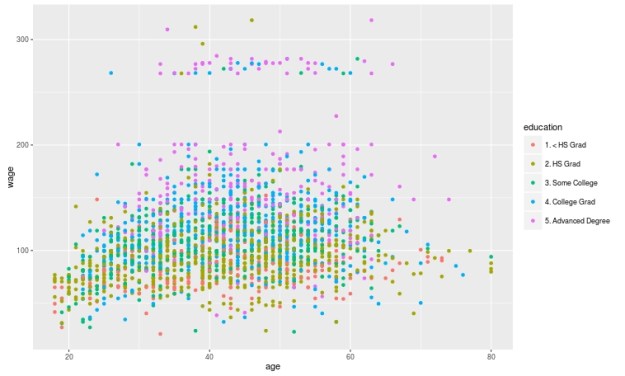Create the Model

We are now going to develop the model for the decision tree. We will use age and wage to predict education as shown in the code below.

TreeModel<-train(education~age+income, method='rpart', data=trainingset)

Create Visual of the Model

We now need to create a visual of the model. This involves installing the package called ‘rattle’. You can install ‘rattle’ separately yourself. After doing this below is the code for the tree model followed by the diagram.

fancyRpartPlot(TreeModel$finalModel)

Rplot02

Here is what the chart means

At the top is node 1 which is called ‘HS Grad” the decimals underneath is the percentage of the data that falls within the “HS Grad” category. As the highest node, everything is classified as “HS grad” until we begin to apply our criteria.
Underneath nod 1 is a decision about wage. If a person makes less than 112 you go to the left if they make more you go to the right.
Nod 2 indicates the percentage of the sample that was classified as HS grade regardless of education. 14% of those with less than a HS diploma were classified as a HS Grade based on wage. 43% of those with a HS diploma were classified as a HS grade based on income. The percentage underneath the decimals indicates the total amount of the sample placed in the HS grad category. Which was 57%.
This process is repeated for each node until the data is divided as much as possible.

Predict

You can predict individual values in the dataset by using the ‘predict’ function with the test data as shown in the code below.

predict(TreeModel, newdata = testingset)

Conclusion

Prediction Trees are a unique feature in data analysis for determining how well data can be divided into subsets. It also provides a visual of how to move through data sequentially based on characteristics in the data.

Z-Scores

Leave a reply

A z-score indicates how closely related one given score is to mean of the sample. Extremely high or low z-scores indicates that the given data point is unusually above or below the mean of the sample.

In order to understand z-scores you need to be familiar with distribution. In general, data is distributed in a bell shape curve. With the mean being the exact middle of the graph as shown in the picture below.

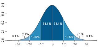
The Greek letter μ is the mean. In this post, we will go through an example that will try to demonstrate how to use and interpret the z-score. Notice that a z-score + 1 takes of 68% of the potential values a z-score + 2 takes of 95%, a z-score + 3 takes of 99%.

Imagine you know the average test score of students on a quiz. The average is 75%. with a standard deviation of 6.4%. Below is the equation for calculating the z-score.

Let’s say that one student scored 52% on the quiz. We can calculate the likelihood for this data point by using the formula above.

(52 – 75) / 6.4 = -3.59

Our value is negative which indicates that the score is below the mean of the sample. Our score is very exceptionally low from the mean. This makes sense given that the mean is 75% and the standard deviation is 6.4%. To get a 52% on the quiz was really bad performance.

We can convert the z-score to a percentage to indicate the probability of getting such a value. To do this you would need to find a z-score conversion table on the internet. A quick glance at the table will show you that the probability of getting a score of 52 on the quiz is less than 1%.

Off course, this is based on the average score of 75% with a standard deviation of 6.4%. A different average and standard deviation would change the probability of getting a 52%.

Standardization

Z-scores are also used to standardize a variable. If you look at our example, the original values were in percentages. By using the z-score formula we converted these numbers into a different value. Specifically, the values of a z-score represent standard deviations from the mean.

In our example, we calculated a z-score of -3.59. In other words, the person who scored 52% on the quiz had a score 3.59 standard deviations below the mean. When attempting to interpret data the z-score is a foundational piece of information that is used extensively in statistics.

Using Regression for Prediction in R

2 Replies

In the last post about R, we looked at plotting information to make predictions. We will now look at an example of making predictions using regression.

We will use the same data as last time with the help of the ‘caret’ package as well. The code below sets up the seed and the training and testing set we need.

> library(caret); library(ISLR); library(ggplot2)
> data("College");set.seed(1)
> PracticeSet<-createDataPartition(y=College$Grad.Rate,  +                                  p=0.5, list=FALSE) > TrainingSet<-College[PracticeSet, ]; TestingSet<- +         College[-PracticeSet, ] > head(TrainingSet)

The code above should look familiar from the previous post.

Make the Scatterplot

We will now create the scatterplot showing the relationship between “S.F. Ratio” and “Grad.Rate” with the code below and the scatterplot.

> plot(TrainingSet$S.F.Ratio, TrainingSet$Grad.Rate, pch=5, col="green", 
xlab="Student Faculty Ratio", ylab="Graduation Rate")

Rplot10

Here is what we did

We used the ‘plot’ function to make this scatterplot. The x variable was ‘S.F.Ratio’ of the ‘TrainingSet’ the y variable was ‘Grad.Rate’.
We picked the type of dot to use using the ‘pch’ argument and choosing ’19’
Next, we chose a color and labeled each axis

Fitting the Model

We will now develop the linear model. This model will help us to predict future models. Furthermore, we will compare the model of the Training Set with the Test Set. Below is the code for developing the model.

> TrainingModel<-lm(Grad.Rate~S.F.Ratio, data=TrainingSet)
> summary(TrainingModel)

How to interpret this information was presented in a previous post. However, to summarize, we can say that when the student to faculty ratio increases one the graduation rate decreases 1.29. In other words, an increase in the student to faculty ratio leads to decrease in the graduation rate.

Adding the Regression Line to the Plot

Below is the code for adding the regression line followed by the scatterplot

> plot(TrainingSet$S.F.Ratio, TrainingSet$Grad.Rate, pch=19, col="green", xlab="Student Faculty Ratio", ylab="Graduation Rate")
> lines(TrainingSet$S.F.Ratio, TrainingModel$fitted, lwd=3)

Rplot01

Predicting New Values

With our model complete we can now predict values. For our example, we will only predict one value. We want to know what the graduation rate would be if we have a student to faculty ratio of 33. Below is the code for this with the answer

> newdata<-data.frame(S.F.Ratio=33)
> predict(TrainingModel, newdata)
      1 
40.6811

Here is what we did

We made a variable called ‘newdata’ and stored a data frame in it with a variable called ‘S.F.Ratio’ with a value of 33. This is x value
Next, we used the ‘predict’ function from the ‘caret’ package to determine what the graduation rate would be if the student to faculty ratio is 33. To do this we told caret to use the ‘TrainingModel’ we developed using regression and to run this model with the information in the ‘newdata’ dataframe
The answer was 40.68. This means that if the student to faculty ratio is 33 at a university then the graduation rate would be about 41%.

Testing the Model

We will now test the model we made with the training set with the testing set. First, we will make a visual of both models by using the “plot” function. Below is the code follow by the plots.

par(mfrow=c(1,2))
plot(TrainingSet$S.F.Ratio,
TrainingSet$Grad.Rate, pch=19, col=’green’, xlab=”Student Faculty Ratio”, ylab=’Graduation Rate’)
lines(TrainingSet$S.F.Ratio, predict(TrainingModel), lwd=3)
plot(TestingSet$S.F.Ratio, TestingSet$Grad.Rate, pch=19, col=’purple’,
xlab=”Student Faculty Ratio”, ylab=’Graduation Rate’)
lines(TestingSet$S.F.Ratio, predict(TrainingModel, newdata = TestingSet),lwd=3)

In the code, all that is new is the “par” function which allows us to see to plots at the same time. We also used the ‘predict’ function to set the plots. As you can see, the two plots are somewhat differ based on a visual inspection. To determine how much so, we need to calculate the error. This is done through computing the root mean square error as shown below.

> sqrt(sum((TrainingModel$fitted-TrainingSet$Grad.Rate)^2))
[1] 328.9992
> sqrt(sum((predict(TrainingModel, newdata=TestingSet)-TestingSet$Grad.Rate)^2))
[1] 315.0409

The main take away from this complicated calculation is the number 328.9992 and 315.0409. These numbers tell you the amount of error in the training model and testing model. The lower the number the better the model. Since the error number in the testing set is lower than the training set we know that our model actually improves when using the testing set. This means that our model is beneficial in assessing graduation rates. If there were problems we may consider using other variables in the model.

Conclusion

This post shared ways to develop a regression model for the purpose of prediction and for model testing.

Simple Prediction

Leave a reply

Prediction is one of the key concepts of machine learning. Machine learning is a field of study that is focused on the development of algorithms that can be used to make predictions.

Anyone who has shopped online at has experienced machine learning. When you make a purchase at an online store, the website will recommend additional purchases for you to make. Often these recommendations are based on whatever you have purchased or whatever you click on while at the site.

There are two common forms of machine learning, unsupervised and supervised learning. Unsupervised learning involves using data that is not cleaned and labeled and attempts are made to find patterns within the data. Since the data is not labeled, there is no indication of what is right or wrong

Supervised machine learning is using cleaned and properly labeled data. Since the data is labeled there is some form of indication whether the model that is developed is accurate or not. If the is incorrect then you need to make adjustments to it. In other words, the model learns based on its ability to accurately predict results. However, it is up to the human to make adjustments to the model in order to improve the accuracy of it.

In this post, we will look at using R for supervised machine learning. The definition presented so far will make more sense with an example.

The Example

We are going to make a simple prediction about whether emails are spam or not using data from kern lab.

The first thing that you need to do is to install and load the “kernlab” package using the following code

install.packages("kernlab")
library(kernlab)

If you use the “View” function to examine the data you will see that there are several columns. Each column tells you the frequency of a word that kernlab found in a collection of emails. We are going to use the word/variable “money” to predict whether an email is spam or not. First, we need to plot the density of the use of the word “money” when the email was not coded as spam. Below is the code for this.

plot(density(spam$money[spam$type=="nonspam"]),
 col='blue',main="", xlab="Frequency of 'money'")

This is an advance R post so I am assuming you can read the code. The plot should look like the following.

Rplot10

As you can see, money is not used to frequently in emails that are not spam in this dataset. However, you really cannot say this unless you compare the times ‘money’ is labeled nonspam to the times that it is labeled spam. To learn this we need to add a second line that explains to us when the word ‘money’ is used and classified as spam. The code for this is below with the prior code included.

plot(density(spam$money[spam$type=="nonspam"]),
 col='blue',main="", xlab="Frequency of 'money'")
lines(density(spam$money[spam$type=="spam"]), col="red")

Your new plot should look like the following

Rplot10

If you look closely at the plot doing a visual inspection, where there is a separation between the blue line for nonspam and the red line for spam is the cutoff point for whether an email is spam or not. In other words, everything inside the arc is labeled correctly while the information outside the arc is not.

The next code and graph show that this cutoff point is around 0.1. This means that any email that has on average more than 0.1 frequency of the word ‘money’ is spam. Below is the code and the graph with the cutoff point indicated by a black line.

plot(density(spam$money[spam$type=="nonspam"]),
 col='blue',main="", xlab="Frequency of 'money'")
lines(density(spam$money[spam$type=="spam"]), col="red")
abline(v=0.1, col="black", lw= 3)

Now we need to calculate the accuracy of the use of the word ‘money’ to predict spam. For our current example, we will simply use in “ifelse” function. If the frequency is greater than 0.1.

We then need to make a table to see the results. The code for the “ifelse” function and the table are below followed by the table.

predict<-ifelse(spam$money > 0.1, "spam","nonspam")
table(predict, spam$type)/length(spam$type)

predict       nonspam        spam
  nonspam 0.596392089 0.266898500
  spam    0.009563138 0.127146273

Based on the table that I am assuming you can read, our model accurately calculates that an email is spam about 71% (0.59 + 0.12) of the time based on the frequency of the word ‘money’ being greater than 0.1.

Of course, for this to be true machine learning we would repeat this process by trying to improve the accuracy of the prediction. However, this is an adequate introduction to this topic.

Survey Design

Leave a reply

Survey design is used to describe the opinions, beliefs, behaviors, and or characteristics of a population based on the results of a sample. This design involves the use of surveys that include questions, statements, and or other ways of soliciting information from the sample. This design is used for descriptive purpose primarily but can be combined with other designs (correlational, experimental) at times as well. In this post, we will look at the following.

Types of Survey Design
Characteristics of Survey Design

Types of Survey Design

There are two common forms of survey design which are cross-sectional and longitudinal. A cross-sectional survey design is the collection of data at one specific point in time. Data is only collected once in a cross-sectional design.

A cross-sectional design can be used to measure opinions/beliefs, compare two or more groups, evaluate a program, and or measure the needs of a specific group. The main goal is to analyze the data from a sample at a given moment in time.

A longitudinal design is similar to a cross-sectional design with the difference being that longitudinal designs require collection over time.Longitudinal studies involve cohorts and panels in which data is collected over days, months, years and even decades. Through doing this, a longitudinal study is able to expose trends over time in a sample.

Characteristics of Survey Design

There are certain traits that are associated with survey design. Questionnaires and interviews are a common component of survey design. The questionnaires can happen by mail, phone, internet, and in person. Interviews can happen by phone, in focus groups, or one-on-one.

The design of a survey instrument often includes personal, behavioral and attitudinal questions and open/closed questions.

Another important characteristic of survey design is monitoring the response rate. The response rate is the percentage of participants in the study compared to the number of surveys that were distributed. The response rate varies depending on how the data was collected. Normally, personal interviews have the highest rate while email request has the lowest.

It is sometimes necessary to report the response rate when trying to publish. As such, you should at the very least be aware of what the rate is for a study you are conducting.

Conclusion

Surveys are used to collect data at one point in time or over time. The purpose of this approach is to develop insights into the population in order to describe what is happening or to be used to make decisions and inform practice.

Simple Regression in R

3 Replies

In this post, we will look at how to perform a simple regression using R. We will use a built-in dataset in R called ‘mtcars.’ There are several variables in this dataset but we will only use ‘wt’ which stands for the weight of the cars and ‘mpg’ which stands for miles per gallon.

Developing the Model

We want to know the association or relationship between the weight of a car and miles per gallon. We want to see how much of the variance of ‘mpg’ is explained by ‘wt’. Below is the code for this.

> Carmodel <- lm(mpg ~ wt, data = mtcars)

Here is what we did

We created the variable ‘Carmodel’ to store are information
Inside this variable, we used the ‘lm’ function to tell R to make a linear model.
Inside the function, we put ‘mpg ~ wt’ the ‘~’ sign means ’tilda’ in English and is used to indicate that ‘mpg’ is a function of ‘wt’. This section is the actual notation for the regression model.
After the comma, we see ‘data = mtcars’ this is telling R to use the ‘mtcar’ dataset.

Seeing the Results

Once you pressed enter you probably noticed nothing happens. The model ‘Carmodel’ was created but the results have not been displayed. Below is various information you can extract from your model.

The ‘summary’ function is useful for pulling most of the critical information. Below is the code for the output.

> summary(Carmodel)

Call:
lm(formula = mpg ~ wt, data = mtcars)

Residuals:
    Min      1Q  Median      3Q     Max 
-4.5432 -2.3647 -0.1252  1.4096  6.8727 

Coefficients:
            Estimate Std. Error t value Pr(>|t|)    
(Intercept)  37.2851     1.8776  19.858  < 2e-16 ***
wt           -5.3445     0.5591  -9.559 1.29e-10 ***
---
Signif. codes:  0 ‘***’ 0.001 ‘**’ 0.01 ‘*’ 0.05 ‘.’ 0.1 ‘ ’ 1

Residual standard error: 3.046 on 30 degrees of freedom
Multiple R-squared:  0.7528,	Adjusted R-squared:  0.7446 
F-statistic: 91.38 on 1 and 30 DF,  p-value: 1.294e-10

We are not going to explain the details of the output (please see simple regression). The results indicate a model that explains 75% of the variance or has an r-square of 0.75. The model is statistically significant and the equation of the model is -5.45x + 37.28 = y

Plotting the Model

We can also plot the model using the code below

> coef_Carmodel<-coef(Carmodel)
> plot(mpg ~ wt, data = mtcars)
> abline(a = coef_Carmodel[1], b = coef_Carmodel[2])

Here is what we did

We made the variable ‘coef_Carmodel’ and stored the coefficients (intercept and slope) of the ‘Carmodel’ using the ‘coef’ function. We will need this information soon.
Next, we plot the ‘mtcars’ dataset using ‘mpg’ and ‘wt’.
To add the regression line we use the ‘abline’ function. To add the intercept and slope we use a = the intercept from our ‘coef_Carmodel’ variable which is subset [1] from this variable. For slope, we follow the same process but use a [2]. This will add the line and your graph should look like the following.

From the visual, you can see that as weight increases there is a decrease in miles per gallon.

Conclusion

R is capable of much more complex models than the simple regression used here. However, understanding the coding for simple modeling can help in preparing you for much more complex forms of statistical modeling.

Experimental Design: Within Groups

1 Reply

Within groups, experimental design is the use of only one group in an experiment. This is in contrast to a between-group design which involves two or more groups. Within-group design is useful when the number of is two low in order to split them into different groups.

There are two common forms of within-group experimental design, time-series, and repeated measures. Under time series there are interrupted times series and equivalent time series. Under repeated-measure, there is only repeated measure design. In this post, we will look at the following forms of within-group experimental design.

interrupted time series
equivalent time series
repeated measures design

Interrupted Time Series Design

Interrupted time series design involves several pre-tests followed by an intervention and then several post-test of one group. By measuring the several times, many threats to internal validity are reduced, such as regression, maturation, and selection. The pre-test results are also used as covariates when analyzing the post-tests.

Equivalent Time Series Design

Equivalent time series design involves the use of a measurement followed by intervention followed by measurement etc. In many ways, this design is a repeated post-test only design. The primary goal is to plot the results of the post-test and determine if there is a pattern that develops over time.

For example, if you are tracking the influence of blog writing on vocabulary acquisition, the intervention is blog writing and the dependent variable is vocabulary acquisition. As the students write a blog, you measure them several times over a certain period. If a plot indicates an upward trend you could infer that blog writing made a difference in vocabulary acquisition.

Repeated Measures

Repeated measures is the use of several different treatments over time. Before each treatment, the group is measured. Each post-test is compared to other post-test to determine which treatment was the best.

For example, let’s say that you still want to assess vocabulary acquisition but want to see how blog writing and public speaking affect it. First, you measure vocabulary acquisition. Next, you employ the first intervention followed by a second assessment of vocabulary acquisition. Third, you use the public speaking intervention followed by the third assessment of vocabulary acquisition. You now have three parts of data to compare

The first assessment of vocabulary acquisition (a pre-test)
The second assessment of vocabulary acquisition (post-test 1 after the blog writing)
The third assessment of vocabulary acquisition (post-test 2 after the public speaking)

Conclusion

Within-group experimental designs are used when it is not possible to have several groups in an experiment. The benefits include needing fewer participants. However, one problem with this approach is the need to measure several times which can be labor intensive.

ANOVA with R

1 Reply

Analysis of variance (ANOVA) is used when you want to see if there is a difference in the means of three or more groups due to some form of treatment(s). In this post, we will look at conducting an ANOVA calculation using R.

We are going to use a dataset that is already built into R called ‘InsectSprays.’ This dataset contains information on different insecticides and their ability to kill insects. What we want to know is which insecticide was the best at killing insects.

In the dataset ‘InsectSprays’, there are two variables, ‘count’, which is the number of dead bugs, and ‘spray’ which is the spray that was used to kill the bug. For the ‘spray’ variable there are six types label A-F. There are 72 total observations for the six types of spray which comes to about 12 observations per spray.

Building the Model

The code for calculating the ANOVA is below

> BugModel<- aov(count ~ spray, data=InsectSprays)
> BugModel
Call:
   aov(formula = count ~ spray, data = InsectSprays)

Terms:
                   spray Residuals
Sum of Squares  2668.833  1015.167
Deg. of Freedom        5        66

Residual standard error: 3.921902
Estimated effects may be unbalanced

Here is what we did

We created the variable ‘BugModel’
In this variable, we used the function ‘aov’ which is the ANOVA function.
Within the ‘aov’ function we told are to determine the count by the difference sprays that is what the ‘~’ tilde operator does.
After the comma, we told R what dataset to use which was “InsectSprays.”
Next, we pressed ‘enter’ and nothing happens. This is because we have to make R print the results by typing the name of the variable “BugModel” and pressing ‘enter’.
The results do not tell us anything too useful yet. However, now that we have the ‘BugModel’ saved we can use this information to find the what we want.

Now we need to see if there are any significant results. To do this we will use the ‘summary’ function as shown in the script below

> summary(BugModel)
            Df Sum Sq Mean Sq F value Pr(>F)    
spray        5   2669   533.8    34.7 <2e-16 ***
Residuals   66   1015    15.4                   
---
Signif. codes:  0 ‘***’ 0.001 ‘**’ 0.01 ‘*’ 0.05 ‘.’ 0.1 ‘ ’ 1

These results indicate that there are significant results in the model as shown by the p-value being essentially zero (Pr(>F)). In other words, there is at least one mean that is different from the other means statistically.

We need to see what the means are overall for all sprays and for each spray individually. This is done with the following script

> model.tables(BugModel, type = 'means')
Tables of means
Grand mean
    
9.5 

 spray 
spray
     A      B      C      D      E      F 
14.500 15.333  2.083  4.917  3.500 16.667

The ‘model.tables’ function tells us the means overall and for each spray. As you can see, it appears spray F is the most efficient at killing bugs with a mean of 16.667.

However, this table does not indicate the statistically significance. For this we need to conduct a post-hoc Tukey test. This test will determine which mean is significantly different from the others. Below is the script

> BugSpraydiff<- TukeyHSD(BugModel)
> BugSpraydiff
  Tukey multiple comparisons of means
    95% family-wise confidence level

Fit: aov(formula = count ~ spray, data = InsectSprays)

$spray
           diff        lwr       upr     p adj
B-A   0.8333333  -3.866075  5.532742 0.9951810
C-A -12.4166667 -17.116075 -7.717258 0.0000000
D-A  -9.5833333 -14.282742 -4.883925 0.0000014
E-A -11.0000000 -15.699409 -6.300591 0.0000000
F-A   2.1666667  -2.532742  6.866075 0.7542147
C-B -13.2500000 -17.949409 -8.550591 0.0000000
D-B -10.4166667 -15.116075 -5.717258 0.0000002
E-B -11.8333333 -16.532742 -7.133925 0.0000000
F-B   1.3333333  -3.366075  6.032742 0.9603075
D-C   2.8333333  -1.866075  7.532742 0.4920707
E-C   1.4166667  -3.282742  6.116075 0.9488669
F-C  14.5833333   9.883925 19.282742 0.0000000
E-D  -1.4166667  -6.116075  3.282742 0.9488669
F-D  11.7500000   7.050591 16.449409 0.0000000
F-E  13.1666667   8.467258 17.866075 0.0000000

There is a lot of information here. To make things easy, wherever there is a p adj of less than 0.05 that means that there is a difference between those two means. For example, bug spray F and E have a difference of 13.16 that has a p adj of zero. So these two means are really different statistically.This chart also includes the lower and upper bounds of the confidence interval.

The results can also be plotted with the script below

> plot(BugSpraydiff, las=1)

Below is the plot

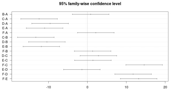
Conclusion

ANOVA is used to calculate if there is a difference of means among three or more groups. This analysis can be conducted in R using various scripts and codes.

Experimental Designs: Between Groups

2 Replies

In experimental research, there are two common designs. They are between and within group design. The difference between these two groups of designs is that between group involves two or more groups in an experiment while within group involves only one group.

This post will focus on between group designs. We will look at the following forms of between group design…

True/quasi-experiment
Factorial Design

True/quasi Experiment

A true experiment is one in which the participants are randomly assigned to different groups. In a quasi-experiment, the researcher is not able to randomly assigned participants to different groups.

Random assignment is important in reducing many threats to internal validity. However, there are times when a researcher does not have control over this, such as when they conduct an experiment at a school where classes have already been established. In general, a true experiment is always considered superior methodological to a quasi-experiment.

Whether the experiment is a true experiment or a quasi-experiment. There are always two groups that are compared in the study. One group is the controlled group, which does not receive the treatment. The other group is called the experimental group, which receives the treatment of the study. It is possible to have more than two groups and several treatments but the minimum for between group designs is two groups.

Another characteristic that true and quasi-experiments have in common is the type of formats that the experiment can take. There are two common formats

Pre- and post test
Post test only

A pre- and post test involves measuring the groups of the study before the treatment and after the treatment. The desire normally is for the groups to be the same before the treatment and for them to be different statistically after the treatment. The reason for them being different is because of the treatment, at least hopefully.

For example, let’s say you have some bushes and you want to see if the fertilizer you bought makes any difference in the growth of the bushes. You divide the bushes into two groups, one that receives the fertilizer (experimental group), and one that does not (controlled group). You measure the height of the bushes before the experiment to be sure they are the same. Then, you apply the fertilizer to the experimental group and after a period of time, you measure the heights of both groups again. If the fertilized bushes grow taller than the control group you can infer that it is because of the fertilizer.

Post-test only design is when the groups are measured only after the treatment. For example, let’s say you have some corn plants and you want to see if the fertilizer you bought makes any difference.in the amount of corn produced. You divide the corn plants into two groups, one that receives the fertilizer (experimental group), and one that does not (controlled group). You apply the fertilizer to the control group and after a period of time, you measure the amount of corn produced. If the fertilized corn produces more you can infer that it is because of the fertilizer. You never measure the corn beforehand because they had not produced any corn yet.

Factorial design involves the use of more than one treatment. Returning to the corn example, let’s say you want to see not only how fertilizer affects corn production but also how the amount of water the corn receives affects production as well.

In this example, you are trying to see if there is an interaction effect between fertilizer and water. When water and fertilizer are increased does production increase, is there no increase, or if one goes up and the other goes down does that have an effect?

Conclusion

Between group designs such as true and quasi-experiments provide a way for researchers to establish cause and effect. Pre- post test is employed as well as factorial designs to establish relationships between variables

Calculating Chi-Square in R

1 Reply

There are times when conducting research that you want to know if there is a difference in categorical data. For example, is there a difference in the number of men who have blue eyes and who have brown eyes. Or is there a relationship between gender and hair color. In other words, is there a difference in the count of a particular characteristic or is there a relationship between two or more categorical variables.

In statistics, the chi-square test is used to compare categorical data. In this post, we will look at how you can use the chi-square test in R.

For our example, we are going to use data that is already available in R called “HairEyeColor”. Below is the data

> HairEyeColor
, , Sex = Male

       Eye
Hair    Brown Blue Hazel Green
  Black    32   11    10     3
  Brown    53   50    25    15
  Red      10   10     7     7
  Blond     3   30     5     8

, , Sex = Female

       Eye
Hair    Brown Blue Hazel Green
  Black    36    9     5     2
  Brown    66   34    29    14
  Red      16    7     7     7
  Blond     4   64     5     8

As you can see, the data comes in the form of a list and shows hair and eye color for men and women in separate tables. The current data is unusable for us in terms of calculating differences. However, by using the ‘marign.table’ function we can make the data useable as shown in the example below.

> HairEyeNew<- margin.table(HairEyeColor, margin = c(1,2))
> HairEyeNew
       Eye
Hair    Brown Blue Hazel Green
  Black    68   20    15     5
  Brown   119   84    54    29
  Red      26   17    14    14
  Blond     7   94    10    16

Here is what we did. We created the variable ‘HairEyeNew’ and we stored the information from ‘HairEyeColor’ into one table using the ‘margin.table’ function. The margin was set 1,2 for the table.

Now all are data from the list are combined into one table.

We now want to see if there is a particular relationship between hair and eye color that is more common. To do this, we calculate the chi-square statistic as in the example below.

> chisq.test(HairEyeNew)

	Pearson's Chi-squared test

data:  HairEyeNew
X-squared = 138.29, df = 9, p-value < 2.2e-16

The test tells us that one or more of the relationships are more common than others within the table. To determine which relationship between hair and eye color is more common than the rest we will calculate the proportions for the table as seen below.

> HairEyeNew/sum(HairEyeNew)
       Eye
Hair          Brown        Blue       Hazel       Green
  Black 0.114864865 0.033783784 0.025337838 0.008445946
  Brown 0.201013514 0.141891892 0.091216216 0.048986486
  Red   0.043918919 0.028716216 0.023648649 0.023648649
  Blond 0.011824324 0.158783784 0.016891892 0.027027027

As you can see from the table, brown hair and brown eyes are the most common (0.20 or 20%) flowed by blond hair and blue eyes (0.15 or 15%).

Conclusion

The chi-square serves to determine differences among categorical data. This tool is useful for calculating the potential relationships among non-continuous variables

Philosophical Foundations of Research: Epistemology

1 Reply

Epistemology is the study of the nature of knowledge. It deals with questions as is there truth and or absolute truth, is there one way or many ways to see something. In research, epistemology manifest itself in several views. The two extremes are positivism and interpretivism.

Positivism

Positivism asserts that all truth can be verified and proven scientifically and can be measured and or observed. This position discounts religious revelation as a source of knowledge as this cannot be verified scientifically. The position of positivist is also derived from realism in that there is an external world out there that needs to be studied.

For researchers, positivism is the foundation of quantitative research. Quantitative researchers try to be objective in their research, they try to avoid coming into contact with whatever they are studying as they do not want to disturb the environment. One of the primary goals is to make generalizations that are applicable in all instances.

For quantitative researchers, they normally have a desire to test a theory. In other words, the develop one example of what they believe is a truth about a phenomenon (a theory) and they test the accuracy of this theory with statistical data. The data determines the accuracy of the theory and the changes that need to be made.

By the late 19th and early 20th centuries, people were looking for alternative ways to approach research. One new approach was interpretivism.

Interpretivism

Interpretivism is the complete opposite of positivism in many ways. Interpretivism asserts that there is no absolute truth but relative truth based on context. There is no single reality but multiple realities that need to be explored and understood.

For interpretist, There is a fluidity in their methods of data collection and analysis. These two steps are often iterative in the same design. Furthermore, intrepretist see themselves not as outside the reality but a player within it. Thus, they often will share not only what the data says but their own view and stance about it.

Qualitative researchers are interpretists. They spend time in the field getting close to their participants through interviews and observations. They then interpret the meaning of these communications to explain a local context specific reality.

While quantitative researchers test theories, qualitative researchers build theories. For qualitative researchers, they gather data and interpret the data by developing a theory that explains the local reality of the context. Since the sampling is normally small in qualitative studies, the theories do not often apply to many.

Conclusion

There is little purpose in debating which view is superior. Both positivism and interpretivism have their place in research. What matters more is to understand your position and preference and to be able to articulate in a reasonable manner. It is often not what a person does and believes that is important as why they believe or do what they do.

Comparing Samples in R

2 Replies

Comparing groups is a common goal in statistics. This is done to see if there is a difference between two groups. Understanding the difference can lead to insights based on statistical results. In this post, we will examine the following statistical test for comparing samples.

t-test/Wilcoxon test
Paired t-test

T-test & Wilcoxon Test

The T-test indicates if there is a significant statistical difference between two groups. This is useful if you know what the difference between the two groups are. For example, if you are measuring height of men and women, if you find that men are taller through a t-test, you can state that gender influences height because the only difference between men and women in this example is their gender.

Below is an example of conducting a t-test in R. In the example, we are looking at if there is a difference in body temperature between beavers who are active versus beavers who are not.

> t.test(temp ~ activ, data = beaver2)

	Welch Two Sample t-test

data:  temp by activ
t = -18.548, df = 80.852, p-value < 2.2e-16
alternative hypothesis: true difference in means is not equal to 0
95 percent confidence interval:
 -0.8927106 -0.7197342
sample estimates:
mean in group 0 mean in group 1 
       37.09684        37.90306

Here is what happened

We use the ‘t.test’ function
Within the ‘t.test’ function we indicate that we want to if there is a difference in ‘temp’ when compared on the factor variable ‘activ’ in the data ‘beaver2’
The output provides a lot of information. The t-stat is -18.58 any number at + 1.96 indicates statistical difference.
Df stands for degrees of freeedom and is used to determine the t-stat and p-value.
The p-value is basically zero. Anything less than 0.05 is considered statistically significant.
Next, we have the 95% confidence interval, which is the range of the difference of the means of the two groups in the population.
Lastly, we have the means of each group. Group 0, the inactive group. had a mean of 37.09684. Group 1. the active group, has a mean of 37.90306.

T-test assumes that the data is normally distributed. When normality is a problem, it is possible to use the Wilcoxon test instead. Below is the script for the Wilcoxon Test using the same example.

> wilcox.test(temp ~ activ, data = beaver2)

	Wilcoxon rank sum test with continuity correction

data:  temp by activ
W = 15, p-value < 2.2e-16
alternative hypothesis: true location shift is not equal to 0

A closer look at the output indicates the same results for the most part. Instead of the t-stat the W-stat is used but the p value is the same for both test.

Paired T-Test

A paired t-test is used when you want to compare how the same group of people respond to different interventions. For example, you might use this for a before and after experiment. We will use the ‘sleep’ data in R to compare a group of people when they receive different types of sleep medication. The script is below

> t.test(extra ~ group, data = sleep, paired = TRUE)

	Paired t-test

data:  extra by group
t = -4.0621, df = 9, p-value = 0.002833
alternative hypothesis: true difference in means is not equal to 0
95 percent confidence interval:
 -2.4598858 -0.7001142
sample estimates:
mean of the differences 
                  -1.58

Here is what happened

We used the ‘t.test’ function and indicate we want to see if ‘extra’ (amount of sleep) is influenced by ‘group’ (two types of sleep medication.
We add the new argument of ‘paired = TRUE’ this tells R that this is a paired test.
The output is the same information as in the regular t.test. The only differences is at the bottom where R only tells you the difference between the two groups and not the means of each. For this example, the people slept about 1 hour and 30 minutes longer on the second sleep medication when compared to the first.

Conclusion

Comparing samples in R is a simple process of understanding what you want to do. With this knowledge, the script and output are not too challenge even for many beginners

Experimental Design: Treatment Conditions and Group Comparision

1 Reply

A key component of experimental design involves making decisions about the manipulation of the treatment conditions. In this post, we will look at the following traits of treatment conditions

Treatment Variables
Experimental treatment
Conditions
Interventions
Outcomes

Lastly, we will examine group comparison.

One of the most common independent variables in experimental design are treatment and measured variables. Treatment variables are manipulated by the researcher. For example, if you are looking at how sleep affects academic performance, you may manipulate the amount of sleep participants receive in order to determine the relationship between academic performance and sleep.

Measured variables are variables that are measured by are not manipulated by the researcher. Examples include age, gender, height, weight, etc.

An experimental treatment is the intervention of the researcher to alter the conditions of an experiment. This is done by keeping all other factors constant and only manipulating the experimental treatment, it allows for the potential establishment of a cause-effect relationship. In other words, the experimental treatment is a term for the use of a treatment variable.

Treatment variables usually have different conditions or levels in them. For example, if I am looking at sleep’s affect on academic performance. I may manipulate the treatment variable by creating several categories of the amount of sleep. Such as high, medium, and low amounts of sleep.

Intervention is a term that means the actual application of the treatment variables. In other words, I broke my sample into several groups and caused one group to get plenty of sleep the second group to lack a little bit of sleep and the last group got nothing. Experimental treatment and intervention mean the same thing.

The outcome measure is the experience of measuring the outcome variable. In our example, the outcome variable is academic performance.

Group Comparison

Experimental design often focuses on comparing groups. Groups can be compared between groups and within groups. Returning to the example of sleep and academic performance, a between group comparison would be to compare the different groups based on the amount of sleep they received. A within group comparison would be to compare the participants who received the same amount of sleep.

Often there are at least three groups in an experimental study, which are the controlled, comparison, and experimental group. The controlled group receives no intervention or treatment variable. This group often serves as a baseline for comparing the other groups.

The comparison group is exposed to everything but the actual treatment of the study. They are highly similar to the experimental group with the experience of the treatment. Lastly, the experimental group experiences the treatment of the study.

Conclusion

Experiments involve treatment conditions and groups. As such, researchers need to understand their options for treatment conditions as well as what types of groups they should include in a study.

Examining Distributions In R

3 Replies

Normal distribution is an important term in statistics. When we say normal distribution, we are speaking of the traditional bell curve concept. Normal distribution is important because it is often an assumption of inferential statistics that the distribution of data points is normal. Therefore, one of the first things you do when analyzing data is to check for normality.

In this post, we will look at the following ways to assess normality.

By graph
By plots
By test

Checking Normality by Graph

The easiest and crudest way to check for normality is visually through the use of histograms. You simply look at the histogram and determine how closely it resembles a bell.

To illustrate this we will use the ‘beaver2’ data that is already loaded into R. This dataset contains five variables “day”, “time”, “temp”, and “activ” for data about beavers. Day indicates what day it was, time indicates what time it was, temp is the temperature of the beavers, and activ is whether the beavers were active when their temperature was taking. We are going to examine the normality of the temperature of active and inactive. Below is the code

> library(lattice)
> histogram(~temp | factor(activ), data = beaver2)

We loaded the ‘lattice’ package. (If you don’t have this package please download)>
We used the histogram function and indicate the variable ‘temp’ then the union ( | ) followed by the factor variable ‘activ’ (0 = inactive, 1 = active)
Next, we indicate the dataset we are using ‘beaver2’
After pressing ‘enter’ you should see the following

As you look at the histograms, you can say that they are somewhat normal. The peaks of the data are a little high in both. Group 1 is more normal than Group 0. The problem with visual inspection is lack of accuracy in interpretation. This is partially solved by using QQ plots.

Checking Normality by Plots

QQplots are useful for comparing your data with a normally distributed theoretical dataset. The QQplot includes a line of a normal distribution and the data points for your data for comparison. The more closely your data follows the line the more normal it is. Below is the code for doing this with our beaver information.

> qqnorm(beaver2$temp[beaver2$activ==1], main = 'Active')
> qqline(beaver2$temp[beaver2$activ==1])

Here is what we did

We used the ‘qqnorm’ function to make the plot
Within the ‘qqnorm’ function we tell are to use ‘temp’ from the ‘beaver2’ dataset.
From the ‘temp’ variable we subset the values that have a 1 in the ‘activ’ variable.
We give the plot a title by adding ‘main = Active’
Finally, we add the ‘qqline’ using most of the previous information.
Below is how the plot should look

Going by sight again. The data still looks pretty good. However, one last test will determine conclusively if the dataset is normal or not.

Checking Normality by Test

The Shapiro-Wilks normality test determines the probability that the data is normally distributed. The lower the probability the less likely that the data is normally distributed. Below is the code and results for the Shapiro test.

> shapiro.test(beaver2$temp[beaver2$activ==1])

	Shapiro-Wilk normality test

data:  beaver2$temp[beaver2$activ == 1]
W = 0.98326, p-value = 0.5583

Here is what happened

We use the ‘shapiro.test’ function for ‘temp’ of only the beavers who are active (activ = 1)
R tells us the p-value is 0.55 or 55%
This means that the probability of our data being normally distributed is 55% which means it is highly likely to be normal.

Conclusion

It is necessary to always test the normality of data before data analysis. The tips presented here provide some framework for accomplishing this.

Characteristics of Experimental Design

1 Reply

In a previous post, we began a discussion on experimental design. In this post, we will begin a discussion on the characteristics of experimental design. In particular, we will look at the following

Random assignment
Control over extraneous variables

Random Assignment

After developing an appropriate sampling method, a researcher needs to randomly assign individuals to the different groups of the study. One of the main reasons for doing this is to remove the bias of individual differences in all groups of the study.

For example, if you are doing a study on intelligence. You want to make sure that all groups have the same characteristics of intelligence. This helps for the groups to equate or to be the same. This prevents people from saying the reason there are differences between groups is because the groups are different and not because of the treatment.

Control Over Extraneous Variables

Random assignment directly leads to the concern of controlling extraneous variables. Extraneous variables are any factors that might influence the cause and effect relationship that you are trying to establish. These other factors confound or confuse the results of a study. There are several methods for dealing with this as shown below

Pretest-posttest
Homogeneous sampling
Covriate
Matching

Pretest-Posttest

A pre-test post-test allows a researcher to compare the measurement of something before the treatment and after the treatment. The assumption is that any difference in the scores of before and after is due to the treatment.Doing the tests takes into account the confounding of the different contexts of the setting and individual characteristics.

Homogeneous Sampling

This approach involves selecting people who are highly similar on the particular trait that is being measured. This removes the problem of individual differences when attempting to interpret the results. The more similar the subjects in the sample are the more controlled the traits of the people are controlled for.

Covariate

Covariates is a statistical approach in which controls are placed on the dependent variable through statistical analysis. The influence of other variables are removed from the explained variance of the dependent variable. Covariates help to explain more about the relationship between the independent and dependent variables.

This is a difficult concept to understand. However, the point is that you use covariates to explain in greater detail the relationship between the independent and dependent variable by removing other variables that might explain the relationship.

Matching

Matching is deliberate, rather than randomly, assigning subject to various groups. For example, if you are looking at intelligence. You might match high achievers in both groups of the study. By placing he achievers in both groups you cancel out there difference.

Conclusion

Experimental design involves the cooperation in random assignment of inclusive differences in a sample. The goal of experimental design is to be sure that the sample groups are mostly the same in a study. This allows for concluding that what happened was due to the treatment.

Experimental Design: A Background

3 Replies

Experimental design is now considered a standard methodology in research. However, this now classic design has not always been a standard approach. In this post, we will the following

The definition of experiment
The history of experiments
When to conduct experiments

Definition

The word experiment is derived from the word experience. When conducting an experiment, the researcher assigns people to have different experiences. He then determines if the experience he assigned people to had some effect on some sort of outcome. For example, if I want to know if the experience of sunlight affects the growth of plants I may develop two different experiences

Experience 1: Some plants receive sunlight
Experience 2: Some plants receive no sunlight

The outcome is the growth of the plants.By giving the plants different experiences of sunlight I can determine if sunlight influences the growth of plants.

History of Experiments

Experiments have been around informally since the 10th century with work done in the field of medicine. The use of experiments as known today began in the early 20th century in the field of psychology. By the 1920’s group comparison became an establish characteristics of experiments. By the 1930’s, random assignment was introduced. By the 1960’s various experimental designs were codified and documented. By the 1980’s there was literature coming out that addressed threats to validity.

Since the 1980’s experiments have become much more complicated with the development of more advanced statistical software problems. Despite all of the new complexity, normally simple experimental designs are easier to understand

When to Conduct Experiments

Experiments are conducted to attempt to establish a cause and effect relationship between independent and dependent variables. You try to create a controlled environment in which you provide the experience or independent variable(s) and then measure how they affect the outcome or dependent variable.

Since the setting of the experiment is controlled. You can say withou a doubt that only the experience influence the outcome. Off course, in reality, it is difficult to control all the factors in a study. The real goal is to try and limit the effect that these other factors have on the outcomes of a study.

Conclusion

Despite their long history, experiments are relatively new in research. This design has grown and matured over the years to become a powerful method for determining cause and effect. Therefore, researchers should e aware of this approach for use in their studies.

Basics of Histograms and Plots in R

1 Reply

R has many fascinating features for creating histograms and plots. In this post, we will only cover some of the most basic concepts of make histograms and plots in R. The code for the data we are using is available in a previous post.

Making a Histogram

We are going to make a histogram of the ‘mpg’ variable in our ‘cars’ dataset. Below is the code for doing this followed by the actual histogram.

Histogram of mpg variable

Here is what we did

We used the ‘hist’ function to create the histogram
Within the hist function we told r to make a histogram of ‘mpg’ variable found in the ‘cars’ dataset.
An additional argument that we added was ‘col’. This argument is used to determine the color of the bars in the histogram. For our example, the color was set to gray.

Plotting Multiple Variables

Before we look at plotting multiple variables you need to make an adjustment to the ‘cyl’ variable in our cars variable. THis variable needs t be changed from a numeric to a factor variable as shown below

cars$cyl<- as.factor(cars$cyl)

Boxplots are an excellent way of comparing groups visually. In this example, we will compare the ‘mpg’ or miles per gallon variable by the ‘cyl’ or number of cylinders in the engine variable in the ‘cars’ dataset. Below is the code and diagram followed by an explanation.

boxplot(mpg ~ cyl, data = cars)

Here is what happened.

We use the ‘boxplot’ function
Within this function we tell are to plot mpg and cyl using the tilda ” ~ ” to tell R to compare ‘mpg’ by the number of cylinders

The box of the boxplot tells you several things

The bottom of the box tells you the 25th percentile
The line in the middle of the box tells you the median
The top of the box tells you the 75th percentile
The bottom line tells you the minimum or lowest value excluding outliers
The top line tells you the maximum or highest value excluding outliers

In order boxplot above, there are three types of cylinders 4, 6, and 8. For 4 cylinders the 25th percentile is about 23 mpg, the 50th percentile is about 26 mpg, while the 75th percentile is about 31 mpg. The minimum value was about 22 and the maximum value was about 35 mpg. A close look at the different blots indicates that four cylinder cars have the best mpg followed by six and finally eight cylinders.

Conclusions

Histograms and boxplots serve the purpose of describing numerical data in a visual manner. Nothing like a picture helps to explain abstract concepts such mean and median.

Qualitative Research Sampling Methods

1 Reply

Qualitative research employs what is generally called purposeful sampling, which is the intentional selection of individuals to better understand the central phenomenon. Under purposeful sampling, there are several ways of selecting individuals for a qualitative study. Below are some examples discussed in this post.

Maximal variation
Extreme case
Theory
Homogeneous
Opportunistic
Snowball

We will also look at suggestions for sample size.

Maximal Variation Sampling

Maximal variation involves selecting individuals that are different on a particular characteristic. For example, if you are doing a study on discrimination, you might select various ethnicities to share their experience with discrimination. By selecting several races you are ensuring a richer description of discrimination.

Extreme Case Sampling

Extreme case sampling involves looking out outliers or unusually situations. For example, studying a successful school in a low-income area may be an example since high academic performance does not normally correlate with low-income areas.

Theory Sampling

Theory sampling involves selecting people based on their ability to help understand theory or process. For example, if you are trying to understand why students drop out of school. You may select dropout students and their teachers to understand the events that lead to dropping out. This technique is often associated with grounded theory.

Homogeneous Sampling

This approach involves selecting several members from the same subgroup. For example, if we are looking at discrimination at a university, we may select only African-American English Majors. Such an example is a clear sub-group of a larger community.

Opportunistic Sampling

Opportunistic sampling is in many ways sampling without a plan or starting with on sampling method and then switching to another because of changes in the circumstances. For example, you may begin with theory sampling as you study the process of dropping out of high school. While doing this, you encounter a student who is dropping out in order to pursue independent studies online. This provides you with the “opportunity” to study an extreme case as well.

Snowball Sampling

Sometimes it is not clear who to contact. In this case, snowball sampling may be appropriate. Snowball sampling is an approach commonly used by detectives in various television shows. You find one person to interview and this same person recommends someone else to talk to. You repeat this process several times until an understanding of the central phenomenon emerges.

Sample Size

Qualitative research involves a much lower sampling size than quantitative. This is for several reasons

You want to provide an in-depth look at one perspective rather than a shallow overview of many perspectives.
The more people involved the harder it is to conduct the analysis.
You want to share the complexities rather than the generalizations of a central phenomenon.

One common rule of thumb is to collect data until saturation is reached. Saturation is when the people in your data begin to say the same things. How long this takes depends and this is by far not an absolute standard.

Conclusion

This is just some of the more common forms of sampling in qualitative research. Naturally, there are other methods and approaches to sampling. The point is that the questions of the study and the context shape the appropriateness of a sampling method.

Analyzing Quantitative Data: Inferential Statistics

1 Reply

In a prior post, we looked at analyzing quantitative data using descriptive statistics. In general, descriptive statistics describe your data in terms of the tendencies within the sample. However, with descriptive stats, you only learn about your sample but you are not able to compare groups nor find the relationship between variables. To deal with this problem, we use inferential statistics.

Types of Inferential Statistics

With inferential statistics, you look at a sample and make inferences about the population. There are many different types of analysis that involve inferential statistics. Below is a partial list. The ones with links have been covered in this blog before.

Pearson Correlation Coefficient–Used to determine the strength of the relationship between two continuous variables
Regression Coefficient-The squared value of the Pearson Correlation Coefficient. Indicates the amount of variance explained between two or more variables
Spearman Rho–Used to determine the strength of the relationship between two continuous variables for non-parametric data.
t-test-Determines if there is a significant statistical difference between two means. The independent variable is categorical while the dependent variable is continuous.
Analysis of Variance-Same as a t-test but for three means or more.
Chi-Square-Goodness-of-Fit-This test determines if there is a difference between two categorical variables.

As you can see, there are many different types of inferential statistical test. However, one thing all test have in common is the testing of a hypothesis. Hypothesis testing has been discussed on this blog before. To summarize, a hypothesis test can tell you if there is a difference between the sample and the population or between the sample and a normal distribution.

One other value that can be calculated is the confidence interval. The confidence interval calculates a range that the results of a statistical test (either descriptive or inferential) can be found. For example, If we that the regression coefficient between two variables is .30 the confidence interval may be between .25 — .40. This range tells us what the value of the correlation would be found in the population.

Conclusion

This post serves as an overview of the various forms of inferential statistics available. Remember, that it is the research questions that determine the form of analysis to conduct. Inferential statistics are used for comparing groups and examining relationships between variables.

Analyzing Quantitative Data: Descriptive Statisitics

4 Replies

For quantitative studies, once you have prepared your data it is now time to analyze it. How you analyze data is heavily influenced by your research questions. Most studies involve the use of descriptive and or inferential statistics to answer the research questions. This post will explain briefly discussed various forms of descriptive statistics.

Descriptive Statistics

Descriptive statistics describe trends or characteristics in the data. There are in general, three forms of descriptive statistics. One form deals specifically with trends and includes the mean, median, and mode. The second form deals with the spread of the scores and includes the variance, standard deviation, and range. The third form deals with comparing scores and includes z scores and percentile rank

Trend Descriptive Stats

Common examples of descriptive statistics that describe trends in the data are mean, median, mode. For example, if we gather the weight of 20 people. The mean weight of the people gives us an idea of about how much each person weighs. The mean is easier to use and remember than 20 individual data points.

The median is the value that is exactly in the middle of a range of several data points. For example, if we have several values arrange from less to greatest such as 1, 4, 7. The number 4 is the median as it is the value exactly in the middle. The mode is the most common number in a list of several values arranged from least to greatest. For example, if we have the values 1, 3, 4, 5, 5, 7. The number 5 is the mode since it appears twice while all the other numbers appear only once.

Spread Scores Descriptive Stats

Calculating spread scores is somewhat more complicated than trend stats. Variance is the average amount of deviation from the mean. It is an average of the amount of error in the data. If the mean of a data set is 5 and the variance is 1 this means that the average departure from the mean of 5 is 1 point.

One problem with variance is that its results are squared. This means that the values of the variance are measured differently than whatever the mean is. To deal with this problem, statisticians square root the results of variance to get the standard deviation. The standard deviation is the average amount that the values in a sample are different from the mean. This value is used in many different statistical analysis.

The range measures the dispersion of the data by subtracting the highest value from the lowest. For example, if the highest value in a data set is 5 and the lowest is 1 the range is 5 – 1 = 4.

Comparison Descriptive States

Comparison descriptive stats are much harder to explain and are often used to calculate more advanced statistics. Two types of comparison descriptive stats include z scores percentile rank.

Z scores tells us how far a data point is from the mean in terms of standard deviation. For example, a z score of 3.0 indicates that this particular data point is 3 standard deviations away from the mean. Z scores are useful in identify outliers and many other things.

The percentile rank is much easier to understand. Percentile rank tells you how many scores fall at or below the percentile. For example, some with a score at the 80th percentile outperformed 80% of the sample.

Conclusion

Descriptive stats are used at the beginning of an analysis. There are many other forms of descriptive stats such as skew, kurtosis, etc. Descriptive stats are useful for making sure your data meets various forms of normality in order to begin inferential statistical analysis. Always remember that your research questions determine what form of analysis to conduct.

Quantitative Data Analysis Preparation

3 Replies

There are many different ways to approach data analysis preparation for quantitative studies. This post will provide some insight into how to do this. In particular, we will look at the following steps in quantitative data analysis preparation.

Scoring the data
Deciding on the types of scores to analyze
Inputting data
Cleaning the data

Scoring the Data

Scoring the data involves the researching assigning a numerical value to each response on an instrument. This includes categorical and continuous variables. Below is an example

Gender: Male(1)____________ Female(2)___________

I think school is boring

Strongly Agree

Agree

Neutral

Disagree

Strongly Disagree

In the example of above, the first item about gender has the value 1 for male and 2 for female. The second item asks the person’s perception of school from 1 being strongly agree all the way to 5 which indicates strongly disagree. Every response was given a numerical value and it is the number that is inputted into the computer for analysis

Determining the Types of scores to Analyze

Once data has been received, it is necessary to determine what types of scores to analyze. Single-item score involves assessing the results from how each individual person responded. An example would be voting, in voting each individual score is add up to determine the results.

Another approach is summed scores. In this approach, the results of several items are added together. This is done because one item alone does not fully capture whatever is being measured. For example, there are many different instruments that measure depression. Several questions are asked and then the sum of the scores indicates the level of depression the individual is experiencing. No single question can accurately measure a person’s depression so a summed score approach is often much better.

Difference scores can involve single-item or summed scores. The difference is that difference scores measure change over time. For example, a teacher might measure a student’s reading comprehension before and after teaching the students basic skills. The difference is then calculated as below

Score 2 – Score 1 = Difference

Inputting Data

Inputting data often happens in Microsoft Excel since it is easy to load an excel file into various statistical programs. In general, inputting data involves giving each item its own column. In this column, you put the respondent’s responses. Each row belongs to one respondent. For example Row 2 would refer to respondent 2. All the results for respondent 2 would be in this row for all the items on the instrument.

If you are summing scores are looking for differences, you would need to create a column to hold the results of the summation or difference calculation. Often this is done in the statistical program and not Microsoft Excel.

Cleaning Data

Cleaning data involves searching for scores that are outside the range of the scale of an item(s) and dealing with missing data. Out range scores can be found through a visual inspection or through running some descriptive statistics. For example, if you have a Lickert scale of 1-5 and one item has a standard deviation of 7 it is an indication that something is wrong because the standard deviation cannot be larger than the range.

Missing data are items that do not have a response. Depending on the type of analysis this can be a major problem. There are several ways o deal with missing data.

Listwise deletion is the removal of any respondent who missed even one item on an instrument
Mean imputation is the inputting of the mean of the variable wherever there is a missing response

There are other more complicated approaches but this provides some idea of what to do.

Conclusion

Preparing data involves planning what you will do. You need to consider how you will score the items, what type of score you will analyze, input the data, and how you will clean it. From here, a deeper analysis is possible.

Test Validity

1 Reply

Validity is often seen as a close companion of reliability. Validity is the assessment of the evidence that indicates that an instrument is measuring what it claims to measure. An instrument can be highly reliable (consistent in measuring something) yet lack validity. For example, an instrument may reliably measure motivation but not valid in measuring income. The problem is that an instrument that measures motivation would not measure income appropriately.

In general, there are several ways to measure validity, which includes the following.

Content validity
Response process validity
Criterion-related evidence of validity
Consequence testing validity
Face validity

Content Validity

Content validity is perhaps the easiest way to assess validity. In this approach, the instrument is given to several experts who assess the appropriateness or validity of the instrument. Based on their feedback, a determination of the validity is determined.

Response Process Validity

In this approach, the respondents to an instrument are interviewed to see if they considered the instrument to be valid. Another approach is to compare the responses of different respondents for the same items on the instrument. High validity is determined by the consistency of the responses among the respondents.

Criterion-Related Evidence of Validity

This form of validity involves measuring the same variable with two different instruments. The instrument can be administered over time (predictive validity) or simultaneously (concurrent validity). The results are then analyzed by finding the correlation between the two instruments. The stronger the correlation implies the stronger validity of both instruments.

Consequence Testing Validity

This form of validity looks at what happened to the environment after an instrument was administered. An example of this would be improved learning due to test. Since the the students are studying harder it can be inferred that this is due to the test they just experienced.

Face Validity

Face validity is the perception that the students have that a test measures what it is supposed to measure. This form of validity cannot be tested empirically. However, it should not be ignored. Students may dislike assessment but they know if a test is testing what the teacher tried to teach them.

Conclusion

Validity plays an important role in the development of instruments in quantitative research. Which form of validity to use to assess the instrument depends on the researcher and the context that he or she is facing.

Quantitative Research Part I

2 Replies

Quantitative research is one of the major forms of research used in the world today. This form of research has several distinct characteristics. In all, there are at least six characteristics of quantitative research and they are listed below.

Description of a research problem
A review of literature that provides justified research problem and questions
Purpose statement that is narrow, observable, and measurable
Collection of numeric data
Statistical analysis
Write up of the results using a standardized format

In this post, we will discuss the first three and look at the next three in a future post.

The Research Problem

The researcher begins by finding a research problem through finding trends in a field or finding something that needs to be explained. An example of a trend would be to assess students’ perception of food services. If the sample does not like the food it can be inferred that the population of the school is disappointed as well.

A different research problem would be to understand the relationship among variables. A variable is a measurable attribute that is studied. For example, a researcher may want to know the relationship between height and weight. He wants to know if an increase in height will lead to an increase in weight.

Review of Literature

The literature review serves two main purposes

Justify the need for the research problem and need
Suggest potential purposes and research questions

The review of literature helps you to find something that has not been studied before or that no one has examined thoroughly. For example, a review of literature might indicate that we know little about how height affects weight. This naturally leads to the question “does height affect weight?” The literature review provides the need for the study as well as helps to shape the research questions.

Research Questions

The research question has already been alluded to. Your goal is to develop specific, narrow, and measurable questions. Specific questions help you to only have a handful of variables you need to deal with. For example, in our height and weight illustration, the question we can ask is “does height influences weight?” In this example, we are looking at two specific variables which are height and weight. We need to measure the height of people and we also need to measure the weight of the same people. We can then use statistics to see if height influences weight. Clear questions are important in clear research design as we will see in the future.

Conclusion

These initial steps are critical to successful research. If the beginning is off and not clear there is no hope for the study. It is at the early stages of a study that students struggle are most frustrated. If a good job is done here the rest of the study is relatively easy to complete.

Share this:

Like this:

Share this:

Like this:

Share this:

Like this:

Share this:

Like this:

Share this:

Like this:

Share this:

Like this:

Share this:

Like this:

Share this:

Like this:

Share this:

Like this:

Share this:

Like this:

Share this:

Like this:

Share this:

Like this:

Share this:

Like this:

Share this:

Like this:

Share this:

Like this:

Share this:

Like this:

Share this:

Like this:

Share this:

Like this:

Share this:

Like this:

Share this:

Like this:

Share this:

Like this:

Share this:

Like this:

Share this:

Like this:

Share this:

Like this:

Share this:

Like this:

Share this:

Like this:

Share this:

Like this:

Share this:

Like this:

Share this:

Like this:

Share this:

Like this:

Share this:

Like this:

Share this:

Like this:

Share this:

Like this:

Share this:

Like this:

Share this:

Like this:

Share this:

Like this:

Share this:

Like this:

Share this:

Like this:

Share this:

Like this:

The Research Problem

Review of Literature