Data visualization plays an important part in explaining an analysis. In this post, we will examine how to make bar graphs using Power BI.


Data visualization plays an important part in explaining an analysis. In this post, we will examine how to make bar graphs using Power BI.
Annotations add text and other objects to a visualization to provide information. The video below explains how to add annotations to a visualization when using Python.

The video below provides two methods that can be used to highlight data points using Python. Which method to use depends on the context, but an analyst should be familiar with both.


In this post, we are going to look at how to highlight data points in a scatterplot. We will specifically look at two different methods for doing this. These two methods are hard coding and programmatically.
Libraries and Data Preparations
First, we will load our libraries and prepare our data. Below are the libraries we will use
import seaborn as sns
import matplotlib.pyplot as plt
from pydataset import data
The first two lines are libraries for our data visualization. The last line of code will be used for pulling the data that we will use. Below we prepare our data by loading it into an object called “df” and we take a quick peek at it as well.
df=data('Prestige')
df.head()
The data set we are using is called “Prestige” and we load it using the data() function. This data contains various jobs, education, income, women, prestige, census, and type information. Next, we will look at how to highlight a specific data point in a scatterplot.
Hard Coding
Hard coding is when you manually pick a specific data point to highlight. Below is the code and output for this
df_prof = df[df.type  ==  'prof']

# Make array orangred for highest income
prof_colors = ['orangered' if (education  ==  12.26) & (income  ==  25879) else 'lightgray'
                  for education,income in zip(df_prof.education, df_prof.income)]

sns.regplot(x = 'education',
            y = 'income',
            data = df_prof,
            fit_reg = False,
            # Send scatterplot argument to color points
            scatter_kws = {'facecolors': prof_colors, 'alpha': 0.7})
plt.show()
We did the following to make the plot above.


Notice the second row and how it is labeled “orangered” this is because this row matches the criteria for the values of education and income. We will use this object to make the colors of our dots
3. The next block of code is for making the visualization. Most of this is self-explanatory. You set your x and y values for education and income,. The fit_reg argument was set to false because we do not want a regression line. The scatter_kws argument is used to set the color of the dots and the alpha sets the level of transparency of the dots.
Setting the highlighted point manually is good if your data is static. However, if your data is dynamic, you want to highlight the points programmatically so that the highlight point changes as the data does.
Progammatically
The code is mostly similar as above with a few minor changes. Below is the code followed by the output and lastly the explanation.
df_prof = df[df.type  ==  'prof']

# Find the highest income
max_income = df_prof.income.max()

# Make a column that denotes which occuaption has highest income
df_prof['point_type'] = ['Highest Income' if income  ==  max_income else 'Others' for income in df_prof.income]

# Encode the hue of the points with the O3 generated column
sns.scatterplot(x = 'education',
                y = 'income',
                hue = 'point_type',
                data = df_prof)
plt.show()
Here is what we did
With this second method, our highlighted data point will change as necessary if it changes in the data.
Conclusion
Highlighting data points is something that is needed at times when creating data visualizations. The examples above provide two different ways to deal with this. Which method is best depends on the context.
The video below explains how to modify the color of glyphs when using Bokeh. Manipulating the color is another way to convey information about your data to the end user.

Modifying the glyphs in a Bokeh data visualization is another useful tool. The video below explains how to do this


In this post, we will examine how to manipulate the color of the glyphs in a Bokeh data visualization. We are doing this not necessarily for aesthetic reasons but to convey additional information. Below are the initial libraries that we need. We will load additional libraries as required.
from pydataset import data
from bokeh.plotting import figure
from bokeh.models import ColumnDataSource
from bokeh.io import output_file, show
pydatasets will be used to load the data we need. The next two lines create the axes we will need and the objects for storing our data. The last line includes functions for saving and displaying our visualization.
Data Preparation
For this example, data preparation is simple. We will load the dataset “Duncan” using the data() function in an object called “df”. This dataset includes data about various occupations as measured on several variables. We will then display the data using the .head() method. Below is the code and output.
df=data('Duncan')
df.head()
Color Glyphs
In the example below, we will color the glyphs based on one of the variables. We will graph education vs income and color code the glyphs based on income. Below is the code followed by the output and finally the explanation.
from bokeh.transform import linear_cmap
from bokeh.palettes import RdBu8

source = ColumnDataSource(data=df)

# Create mapper
mapper = linear_cmap(field_name="income", palette=RdBu8, low=min(df["income"]), high=max(df["income"]))

# Create the figure
fig = figure(x_axis_label="Education", y_axis_label="Income", title="Education vs. Income")

# Add circle glyphs
fig.circle(x="education", y="income", source=source, color=mapper,size=16)

output_file(filename="education_vs_income.html")
show(fig)
Here is what we did
You could set the glyph color to a third variable, which would allow you to express a third variable in a two-dimensional space. For example, we could have used the “prestige” variable for the coloring of the glyphs rather than income, as income was already represented on the y-axis.
Adding a Color Bar
Adding a color bar will help to explain to a reader of our visualization what the color of the glyphs means. The code below is mostly the same and is followed by the output and lastly the explanation.
from bokeh.models import ColorBar
source = ColumnDataSource(data=df)

# Create mapper
mapper = linear_cmap(field_name="income", palette=RdBu8, low=min(df["income"]), high=max(df["income"]))

# Create the figure
fig = figure(x_axis_label="Education", y_axis_label="Income", title="Education vs. Income")
fig.circle(x="education", y="income", source=source, color=mapper,size=16)

# Create the color_bar
color_bar = ColorBar(color_mapper=mapper['transform'], width=8)

# Update layout with color_bar on the right
fig.add_layout(color_bar, "right")
output_file(filename="Education_vs_prestige_color_mapped.html")
show(fig)
Here is what happened.
There is one more example of glyph manipulation below.
Color by Category
In this last example, we will map an additional categorical variable onto our plot using color. Below is the code, output, and explanation.
# Import modules
from bokeh.transform import factor_cmap
from bokeh.palettes import Category10_5
source = ColumnDataSource(data=df)

# Create positions
TOOLTIPS=[('Education', '@education'), ('Prestige', '@prestige')]
positions = ["wc","bc","prof"]
fig = figure(x_axis_label="Education", y_axis_label="Prestige", title="Education vs Prestige", tooltips=TOOLTIPS)

# Add circle glyphs
fig.circle(x="education", y="prestige", source=source, legend_field="type",
           size=16,fill_color=factor_cmap("type", palette=Category10_5, factors=positions))

output_file(filename="Education_vs_prestige_by_type.html")
show(fig)
Conclusion
Bokeh allows you to do many cool things when creating a visualization for data purposes. This post was focused on how to manipulate the glyphs in a scatterplot. However, there is so much more that can be done beyond what was shared here.
The video below shows you how to make multiple plots with Bokeh. This is a valuable tool when you are trying to develop multiple visualizations for comparison purposes.

In the video below, we will take a look at Bokeh tools and tooltips in Python. Tools and tooltips are great options for modifying your data visualization’s interactivity.


In this post, we will examine how to modify the default display of a plot in Bokeh, a library for interactive data visualizations in Python. Below are the initial libraries that we need.
from pydataset import data
from bokeh.plotting import figure
from bokeh.io import output_file, show
The first line of code is where our data comes from. We are using the data() function from pydataset for loading our data. The next two lines are for making the plot’s figure (x and y axes) and for the output file.
Data Preparation
There is no data preparation beyond loading the dataset using the data() function. We pick the dataset “Duncan” and load it into an object called “df.” The code is below, followed by a brief view of the actual data using the .head() method.
df=data('Duncan')
df.head()
This dataset includes various occupations measured in four ways: job type, income, education, and prestige.
Default Graph’s Appearance
Before we modify the appearance of the plot, it is important to know what the default appearance of the plot is for comparison purposes. Below is the code for a simple plot followed by the actual output and then lastly an explanation.
# Create a new figure
fig = figure(x_axis_label="Education", y_axis_label="Income")

# Add circle glyphs
fig.circle(x=df["education"], y=df["income"])

# Call function to produce html file and display plot
output_file(filename="my_first_plot.html")
show(fig)
The first line of code sets up the fig or figure. We use the figure() function to label the axes which are education and income. The second line of code creates the actual data points in the figure using the .circle() method. The last two lines create the output and display it.

So the figure above is the default appearance of a graph. Below we will look at several modifications.
Modification 1
In the code below, we are making the following changes to the plot.
Below is the code followed by the output and the explanation
# Import curdoc
from bokeh.io import curdoc

prof = df.loc[df["type"] == "prof"]
bc = df.loc[df["type"] == "bc"]

# Change theme to contrast
curdoc().theme = "contrast"
fig = figure(x_axis_label="Education", y_axis_label="Income")

# Add prof circle glyphs
fig.circle(x=prof["education"], y=prof["income"], color="yellow", legend_label="prof",size=10)

# Add bc circle glyphs
fig.circle(x=bc["education"], y=bc["income"], color="red", legend_label="bc",size=10)

output_file(filename="prof_vs_bc.html")
show(fig)
Here is what happened,
You can see the difference between this second plot and the first one. This also shows the flexibility that is inherent in the use of Bokeh. Below we add one more variation to the display.
Modified Graph’s Appearance
The plot below is mostly the same except for the following
Below is the code followed by the graph and the explanation
# Create figure
wc = df.loc[df["type"] == "wc"]
prof = df.loc[df["type"] == "prof"]
bc = df.loc[df["type"] == "bc"]

fig = figure(x_axis_label="Education", y_axis_label="Income")

# Add circle glyphs for houses
fig.circle(x=wc["education"], y=wc["income"], legend_label="wc", color="purple",size=10)

# Add square glyphs for units
fig.square(x=prof["education"], y=prof["income"], legend_label="prof", color="red",size=10)

# Add triangle glyphs for townhouses
fig.triangle(x=bc["education"], y=bc["income"], legend_label="bc", color="green",size=10)

output_file(filename="education_vs_income_by_type.html")
show(fig)
The code is almost all the same. The main difference is there are now three job types and each type has a different shape for their data points. The shapes are determined by using either .circle(), .triangle(), or .square() methods.
Conclusion
There are many more ways to modify the appearance of visualization in bokeh. The goal here was to provide some basic examples that may lead to additional exploration.


In this post, we will look at how to manipulate the different tools and tooltips that you can use to interact with data visualizations that are made using Bokeh in Python. Tool are the icons that are displayed by default to the right of a visual when looking at a Bokeh output. To the right is what default tools look like. Tooltips provide interactive data based on the position of the mouse.
We will now go through the process of changing these tools and tooltips for various reasons and purposes.
Load Libraries
First, we need to load the libraries we need to make our tools. Below is the code followed by an explanation.
from pydataset import data
from bokeh.plotting import figure
from bokeh.io import output_file, show
We start by loading “data” from “pydataset”. This library contains the actual data we are going to use. The other libraries are all related to Bokeh’s “figure” which will create details for our visualization. In addition, we will need the “output_file” to make our HTML document and the “show” function to display our visualization.
Data Preparation
Data preparation is straightforward. All we have to do is load our data into an object. We will use the “Duncan” dataset, which contains data on various jobs’ income, education, and prestige. Below is the code followed by a snippet of the actual data.
df=data('Duncan')
df.head()
Default Settings for Tools
We will now look at a basic plot with the basic tools. Below is the code.
# Create a new figure
fig = figure(x_axis_label="income", y_axis_label="prestige")

# Add circle glyphs
fig.circle(x=df["income"], y=df["prestige"])

# Call function to produce html file and display plot
output_file(filename="my_first_plot.html")
show(fig)
There is nothing new here. We create the figure for our axes first. Then we add the points in the next line of code. Lastly, we write some code to create an output. The default tools has 7 options. Below they are explained from top to bottom.
We will now show how to customize the available tools.
Custom Settings for Tooltips
In order to make a set of custom tools, we need to make some small modifications to the previous code as shown below.
# Create a list of tools
tools = ["lasso_select", "wheel_zoom", "reset","save"]

# Create figure and set tools
# Create a new figure
fig = figure(x_axis_label="income", y_axis_label="prestige",tools=tools)

# Add circle glyphs
fig.circle(x=df["income"], y=df["prestige"])

# Call function to produce html file and display plot
output_file(filename="my_first_plot.html")
show(fig)
What is new in the code is the object called “tools”. This object contains a list of the tooltips we want to be available in our plot. The names of the tools is available in the Bokeh documentation. We then add this object “tools” to the argument called “tools” in the line of code where we create the “fig” object. If you compare the second plot to the first plot you can see we have fewer tools in the second one as determine by our code.
Hover Tooltip
The hover tooltip allows you to place your mouse over the plot and have information displayed about what your mouse is resting upon. Being able to do this can be useful for gaining insights about your data. Below is the code and the output followed by an explanation.
# Import ColumnDataSource
from bokeh.models import ColumnDataSource

# Create source
source = ColumnDataSource(data=df)

# Create TOOLTIPS and add to figure
TOOLTIPS = [("Education", "@education"), ("Position", "@type"), ("Income", "@income")]
fig = figure(x_axis_label="education", y_axis_label="income", tooltips=TOOLTIPS)

# Add circle glyphs
fig.circle(x="education", y="income", source=source)
output_file(filename="first_tooltips.html")
show(fig)
Here is what happened.
Conclusion
With tooltips and tools you can make some rather professional looking visualization with a minimum amount of code. That is what makes the Bokeh library so powerful.
The video below provides an introduction to making bar graphs using the Bokeh library and Python.

Bokeh is a data visualization library available in Python with the unique ability of interaction. In this video, we will look at how to make a basic bar graph using bokeh.
To begin we need to load certain libraries as shown below.
from pydataset import data
import pandas as pd
from bokeh.plotting import figure
from bokeh.io import output_file, show
In the code above, we load the “pydataset” library to gain access to the data we will use. Next, we load “pandas” which will help us with some data preparation. The last two libraries are related to “bokeh.” The “figure” function will be used to set the actual plot, the “output_file” function will allow us to save our plot as an HTML file and the “show” function will allow us to display our plot.
Data Preparation
We need to do two things to be ready to create our bar graph. First, we need to load the data. Second, we need to calculate group means for the bar graph. Below is the code for the first step followed by the output.
df=data('Duncan')
df.head()
In the code above we use the “data” function to load the “Duncan” dataset into an object called “df”. Next, we display the output of this. The “Duncan” dataset contains data on different jobs, the type of job, income, education, and prestige. We want to graph prestige and job type as a bar graph which will require us to calculate the mean of prestige by type. The code for this is below.
# Calculate group means of prestige
positions = df.groupby('type', as_index=False)['prestige'].mean()
positions
In the code above we use the “groupby” function on the “df” object. Inside the function, we indicate we want to group by “type”. The “as_index” argument is set to false so that the “type” column is not set at the index or you can say as the row numbers. Next, we subset the data using square brackets to only include the “prestige” column. Lastly, we indicate that we want to calculate the “mean”. The result is that there are three job types and we have the mean for each job’s prestige. The job types and means from this table above are what we will use for making our visualization.
Bar Graph
We are now ready to make our bar graph. Below is the code followed by the output.
# Instantiate figure
fig = figure(x_axis_label="positions", y_axis_label="Prestige", x_range=positions["type"])

# Add bars
fig.vbar(x=positions["type"], top=positions["prestige"],width=0.9)

# Produce the html file and display the plot
output_file(filename="Prestige.html")
show(fig)
Here are the steps.
Conclusion
Bokeh has lots of cool tools available for the data analyst. This post was focused on bar graphs but this is only the most basic information that has been shared here. There is much more possible with this library.

Bokeh is another data visualization library available in Python. One of Bokeh’s unique features is that it allows for interaction. In this post, we will learn how to make a basic scatterplot in Bokeh while also exploring some of the basic interactions that are provided by default.
Data Preparation
We are going to make a scatterplot using the “Duncan” data set that is available in the “pydataset” library. Below is the initial code.
from pydataset import data
from bokeh.plotting import figure
from bokeh.io import output_file, show
The code above is just the needed libraries. We loaded “pydataset” because this is where our data will come from. All of the other libraries are related to “bokeh.” “Figure” allows us to set up our axes for the scatterplot. “Output_file” allows us to create the file of our plot. Lastly, “show” allows us to show the plot of our visualization. In the code below we will load our dataset, give it a name, and print the first few rows.
df=data('Duncan')
df.head()
In the code above we store the “Duncan” dataset in an object called “df” using the data() function. We then display a snippet of the data using the .head() function. The “Duncan” data shares information on jobs as defined by several variables. We will now proceed
Making the Scatterplot
We will now make our scatterplot. We have to do this in three steps.
Below is the code with the output
# Create a new figure
fig = figure(x_axis_label="education", y_axis_label="income") #labels axises

# Add circle glyphs
fig.circle(x=df["education"], y=df["income"]) #adds the dots

# Call function to produce html file and display plot
output_file(filename="my_first_plot.html")
show(fig)
At the top of the code, we create our axis information using the “figure” function. Here we are plotting education vs income and storing all of this in an object called “fig”. Next, we insert the data into our plot using the “circle” function. To insert the data we also have to subset the “df” dataframe for the variables that we want. Note that the data added to a plot are called “glyphs” in Bokeh. Lastly, we create an output file using a function with the same name and show the results.
To the right of your plot, there are also some interaction buttons as shown below

Here is what they do from top to bottom.
There are other interactions possible but these are the default ones when you make a plot.
Conclusion
Bokeh is one of many tools used in Python for data visualization. It is a powerful tool that can be used in certain contexts. The interactive tools can also enhance the user experience.
The video below provides an explanation of how to create dropdown and check boxes for visuals using Plotly in R.


Linking plots involves allowing the action you take in one plot to affect another. Doing this can allow the user to uncover various patterns that may not be apparent otherwise. Using plotly, it is possible to link plots and this is shown in the video below.


It is possible to animate your visualizations in R using Plotly. The video below provides some tips for how to make animations a reality in your visualizations.

Making scatterplots is a part of the data analyst’s life. The video below shows how a scatterplot can be created using ploty in the R environment.


The video below provides examples of how to make bar graphs using plotly in R.


Plotly is a library that allows you to make interactive charts in R. The example in the video below will focus on making histograms with this library.

Matplotlib is a data visualization module used often in Python. In this video, we will go over some introductory basic commands. Doing so will allow anybody who wants to be able to make simple manipulations to their visualizations.

Principal component analysis is a tool for reducing the number of variables in a dataset without losing too much information. This is a great way to summarize information or to simplify things for a more complex analysis. The video provides a simple example of how to do this.

Python has a great library called that Altair that makes it really easy to make various data visualizations. The primary strength of this particular library is how easy it is to use and to also create interactive plots. The video below provides an introduction to using this innovative tool.


We are going to take a look at Altair which is a data visulization library for Python. What is unique abiut Altair compared to other packages experienced on this blog is that it allows for interactions.

The interactions can take place inside jupyter or they can be exported and loaded onto websites as we shall see. In the past, making interactions for website was often tught using a jacascript library such as d3.js. D3.js works but is cumbersome to work with for the avaerage non-coder. Altair solves this problem as Python is often seen as easier to work with compared to javascript.
Installing Altair
If Altair is not already install on your computer you can do so with the following code
pip install altair vega_datasets

OR

conda install -c conda-forge altair vega_datasets
Which one of the lines above you use will depend on the type of Python installation you have.
Goal
We are going to make some simple visualizations using the “Duncan” dataset from the pydataset library using Altair. If you do not have pydataset install on your ocmputer you can use the code listed above to install it. Simple replace “altair vega_datasets” with “pydataset.” Below is the initial code followed by the output
import pandas as pd
from pydataset import data
df=data("Duncan")
df.head()
In the code above, we load pandas and import “data” from the “pydataset” library. Next, we load the “Duncan” dataset as the object “df”. Lastly, we use the .head() function to take a look at the dataset. You can see in the imagine above what variables are available.
Our first visualization is a simple bar graph. The code is below followed by the visualization.
import altair as alt
alt.Chart(df).mark_bar().encode(
x= "type",
y = "prestige"
)
In the code above we did the following,
The three dots in the upper right provide options for saving or editing the plot. We will learn more about saving plots later. In addition, Altair follows the grammar of graphics for creating plots. This has been discussed in another post but a summary of the components are below.
We will not deal with all of these but we have dealt with the following
In our second example, we will make a scatterplot. The code and output are below.
alt.Chart(df).mark_circle().encode(
x= "education",
y = "prestige"
)
The code is mostly the same. We simple use .mark_circle() as to indicate the type of geometric object. For .encode() we made sure to use two continuous variables.
In the next plot, we add a categorical variable to the scatterplot by manipulating the color.
alt.Chart(df).mark_circle().encode(
    x= "education",
    y = "prestige",
    color='type'
)
The only change is the addition of the “color”argument which is set to the categorical vareiable of “type.”
It is also possible to use bubbles to indicate size. In the plot below we can add the income varibale to the plot using bubbles.
alt.Chart(df).mark_circle().encode(
    x= "education",
    y = "prestige",
    color='type',
    size="income"
)
The latest argument that was added was the “size” argument which was used to map income to the plot.
You can also facet data by piping. The code below makes two plots and saving them as objects. Then you print both by typing the name of the objects while separated by the pipe symbol (|) which you can find above the enter key on your keyboard. Below you will find two different plots created through this piping process.
educationPlot=alt.Chart(df).mark_circle().encode(
    x= "education",
    y = "prestige",
    color='type',
)
incomePlot=alt.Chart(df).mark_circle().encode(
    x= "income",
    y = "prestige",
    color='type',
)
educationPlot | incomePlot
With this code you can make multiple plots. Simply keep adding pipes to make more plots.
Interaction and Saving Plots
It is also possible to move plots interactive. In the code below we add the command called tool tip. This allows us to add an additional variable called “income” to the chart. When the mouse hoovers over a data-point the income will display.
However, since we are in a browser right now this will not work unless w save the chart as an html file. The last line of code saves the plot as an html file and renders it using svg. We also remove the three dots in the upper left corner by adding the ‘actions’:False. Below is the code and the plot once the html was loaded to this blog.
interact_plot=alt.Chart(df).mark_circle().encode(
    x= "education",
    y = "prestige",
    color='type',
    tooltip=["income"]
)
interact_plot.save('interact_plot.html',embed_options={'renderer':'svg','actions':False})
I’ve made a lot of visuals in the past and never has it been this simple
Conclusion
Altair is another tool for visualizations. This may be the easiest way to make complex and interactive charts that I have seen. As such, this is a great way to achieve goals if visualizing data is something that needs to be done.

It is common in research to want to visualize data in order to search for patterns. When the number of features increases, this can often become even more important. Common tools for visualizing numerous features include principal component analysis and linear discriminant analysis. Not only do these tools work for visualization they can also be beneficial in dimension reduction.
However, the available tools for us are not limited to these two options. Another option for achieving either of these goals is t-Distributed Stochastic Embedding. This relative young algorithm (2008) is the focus of the post. We will explain what it is and provide an example using a simple dataset from the Ecdat package in R.
t-sne is a nonlinear dimension reduction visualization tool. Essentially what it does is identify observed clusters. However, it is not a clustering algorithm because it reduces the dimensions (normally to 2) for visualizing. This means that the input features are not longer present in their original form and this limits the ability to make inference. Therefore, t-sne is often used for exploratory purposes.
T-sne non-linear characteristic is what makes it often appear to be superior to PCA, which is linear. Without getting too technical t-sne takes simultaneously a global and local approach to mapping points while PCA can only use a global approach.
The downside to t-sne approach is that it requires a large amount of calculations. The calculations are often pairwise comparisons which can grow exponential in large datasets.
We will use the “Rtsne” package for the analysis, and we will use the “Fair” dataset from the “Ecdat” package. The “Fair” dataset is data collected from people who had cheated on their spouse. We want to see if we can find patterns among the unfaithful people based on their occupation. Below is some initial code.
library(Rtsne)
library(Ecdat)To prepare the data, we first remove in rows with missing data using the “na.omit” function. This is saved in a new object called “train”. Next, we change or outcome variable into a factor variable. The categories range from 1 to 9
Below is the code.
train<-na.omit(Fair)
train$occupation<-as.factor(train$occupation)Before we do the analysis we need to set the colors for the different categories. This is done with the code below.
colors<-rainbow(length(unique(train$occupation)))
names(colors)<-unique(train$occupation)
We can now do are analysis. We will use the “Rtsne” function. When you input the dataset you must exclude the dependent variable as well as any other factor variables. You also set the dimensions and the perplexity. Perplexity determines how many neighbors are used to determine the location of the datapoint after the calculations. Verbose just provides information during the calculation. This is useful if you want to know what progress is being made. max_iter is the number of iterations to take to complete the analysis and check_duplicates checks for duplicates which could be a problem in the analysis. Below is the code.
tsne<-Rtsne(train[,-c(1,4,7)],dims=2,perplexity=30,verbose=T,max_iter=1500,check_duplicates=F)## Performing PCA
## Read the 601 x 6 data matrix successfully!
## OpenMP is working. 1 threads.
## Using no_dims = 2, perplexity = 30.000000, and theta = 0.500000
## Computing input similarities...
## Building tree...
## Done in 0.05 seconds (sparsity = 0.190597)!
## Learning embedding...
## Iteration 1450: error is 0.280471 (50 iterations in 0.07 seconds)
## Iteration 1500: error is 0.279962 (50 iterations in 0.07 seconds)
## Fitting performed in 2.21 seconds.Below is the code for making the visual.
plot(tsne$Y,t='n',main='tsne',xlim=c(-30,30),ylim=c(-30,30))
text(tsne$Y,labels=train$occupation,col = colors[train$occupation])
legend(25,5,legend=unique(train$occupation),col = colors,,pch=c(1))
You can see that there are clusters however, the clusters are all mixed with the different occupations. What this indicates is that the features we used to make the two dimensions do not discriminant between the different occupations.
Conclusion
T-SNE is an improved way to visualize data. This is not to say that there is no place for PCA anymore. Rather, this newer approach provides a different way of quickly visualizing complex data without the limitations of PCA.

Network visualizations involve displaying interconnected nodes commonly associated with social networks. D3.js has powerful capabilities to create these visualizations. In this post, we will learn how to make a simple force-directed graph.
A force directed graph uses an algorithm that spaces the nodes in the graph away from each other based on a value you set. There are several different ways to determine how the force influences the distance of the nodes from each other that will be explored somewhat in this post.

The Data
To make the visualization it is necessary to have data. We will use a simple json file that has nodes and edges. Below is the code
{

"nodes": [

{ "name": "Tom" },

{ "name": "Sue" },

{ "name": "Jina" },

{ "name": "Soli" },

{ "name": "Lala" }

],

"edges": [

{ "source": 0, "target": 1 },

{ "source": 0, "target": 4 },

{ "source": 0, "target": 3 },

{ "source": 0, "target": 4 },

{ "source": 0, "target": 2 },

{ "source": 1, "target": 2 }

]

}
The nodes in this situation will represent the circles that we will make. In this case, the nodes have names. However, we will not print the names in the visualization for the sake of simplicity. The edges represent the lines that will connect the circles/nodes. The source number is the origin of the line and the target number is where the line ends at. For example, “source: 0” represents Tom and “Target”: 1 means draw a line from Tom to Sue.
Setup
To begin the visualization we have to create the svg element inside our html doc. Lines 6-17 do this as shown below.

Next, we need to create the layout of the graph. The .node() and the .link() functions affect the location of the nodes and links. The .size() affects the gravitational center and initial position of the visualization. There is also some code that is commented out in below that will be discussed later. Below are lines 18-25 of our code.

Now we can write the code that will render or draw our object. We need to append the edges and nodes, indicate color for both, as well as the radius of the circles of the nodes. All of this is captured in lines 26-44

The final step is to handle the ticks. To put it simply, the ticks handles recalculating the position of the nodes. Below is the code for this.

We can finally see are visual as shown below
You can clearly see that the nodes are on top of each other. This is because we need to adjust the use of the force in the force-directed graph. There are many ways to adjust this, but we will look at two functions. These are .linkDistance() and .charge().
The .linkDistance() function indicates how far nodes are from each other at the end of the simulation. To add this to our code you need to remove the comments on line22 as shown below.

Below is an update of what our visualization looks like.
Things are better but the nodes are still on top of each other. The real differences is that the edges are longer. To fix this, we need to use the .charge() function. The .charge() function indicates how much nodes are attracted to each other or repel each other. To use this function you need to remove the comments on line 23 as shown below.

The negative charge will cause the nodes to push away from each other. Below is what this looks like.
You can see that as the nodes were moved around the stayed far from each other. This is because of the negative charge. Off course, there are other ways to modify this visualization but this is enough for now.
Conclusion
Force-directed graphs are a powerful tool for conveying what could be a large amount of information. This post provided some simple ways that this visualization can be developed and utilized for practical purposes.

Pie charts are one of many visualizations that you can create using D3.js. We are going to learn how to do the following in this post.
Most of these examples require just a minor adjustment in a standard piece of code. This will make more sense in a minute.
Make a Circle
Making a circle involves using the .arc() method. In this method there are four parameters that you manipulate to get different shapes. They are explained below
Therefore, to make several different shapes we manipulate these different parameters. In the code below, we create the svg element first (lines 7-10) then our circle (lines 11-15). Lastly, we append the path to the svg element (lines 16-21). Below is the code and picture.


The rest of the examples primarily deal with manipulating the existing code.
Donut
To make the donut, you need to change the value inside the .innerRadius() parameter. The larger the value the bigger the hole in the middle of the circle will become. In order to generate the donut below you need to change the value found in line 12 of the code to 100.

Pie Wedge
To make a wedge you need to replace lines 14-15 of the code with the following
.startAngle(0*Math.PI * 2/360)

.endAngle(90*Math.PI * 2/360);
This is telling d3.js to start the angle at 0 degrees and stop at 90 degrees. This is another way of saying making a wedge of 1/4 of the circle. Doing this will create the following.

Segment
In order to make the segment you keep the code the same as above for the pie wedge but at a change to the .innerRadius() parameter. AS shown below,
.innerRadius(100)

.outerRadius(170)

.startAngle(0*Math.PI * 2/360)

.endAngle(90*Math.PI * 2/360);

Pie Chart
A pie chart is just a more complex version of what we have already done. You still need to set up your svg element. This is don in lines 7-14. Notice that we also had to add a g element and a transform attribute.
Line 16 contains the data for making the pie chat. This is hard coded but we can also use other forms of data. Line 17 uses the .pie() method with the data to set the stage for our pie chart.
Lines 19-27 are for generating the arc. This code is mostly the same except for the functions that are used for the .startAngle() and .end Angle() methods. Line 29 sets the color and Lines 30-42 draw the paths for creating the image. The code with the // will be explained in a moment. Below is the code and the pie chart.


Pie Chart Variation
Below is the same pie chart but with some different features.
Below is the pie chart

You can perhaps now see that the possibilities are endless with this.
Conclusion
Pie charts and their related visualizations are another option for communicating insights of data

Dendrogram is a type of hierarchical visualization commonly used in data science with hierarchical clustering. In d3.js, the dendrogram looks slightly different in that the root is in the center and the nodes branch out from there. This idea continues for every parent child relationship in the data.
In this post, we will make a simple dendrogram with d3.js using a simple json file shown below.
{

  "name": "President",

          "children": [

        { "name": "VP of Academics",

        "children":[

          {"name":"Dean of Psych"},

          {"name":"Dean of Ed"}

        ] },

       { "name": "VP of Finance" },

        { "name": "VP of Students" }

      ]

    }
You will need to save the code above as a json file if you want to make this example. In the code, this json example is called “university.json”
Making the Dendrogram

In lines 20-26, the radius of the nodes is set and added to the svg element. The clusters are set with the creation of the cluster variable. Below is the code.

In lines 27-37, we set the position of the nodes and links as well as diagonals for the path.

Lines 49-80, have three main blocks of code.
The first block creates a variable called nodesGroups. This code provides a place to hold the nodes and the text that we are going to create.
The second block of code is adding circles to the nodeGroups with additional settings for the color and radius size. Lastly, the third block of code adds texts to the nodesGroups.

When all the steps have been taken, you will see the following when you run the code.

You can see how things worked. The center is the president with the vp of academics of to the right. The president has three people under him (all VPs) while the VP of academics has two people under him (deans). The colors for the path and the circle are all set in the last block of code that was discussed.
Conclusion
Dendrograms allow you to communicate insights about data in a distinctly creative way. This example was simplistic but serves the purpose of exposing you to another way of using d3.js

D3.js has the ability to draw rather complex shapes using techniques called path generators. This will allow you to many things that would otherwise be difficult when working with visualizations.
In this post, we will look at three different examples of path generation involving d3.js. The three examples are as follows
Making a Triangle
To make a triangle we start by appending a svg to the body element of our document (lines 7-12). Then when create an array that has three coordinates. We need three coordinates because that is how many coordinates a triangle needs (lines 13-17). After this, we create a variable called generate and use the .svg.line() method to draw the actual lines that we want (lines 18-20).
After this, we append the data and other characteristics to the svg variable. This allows us to set the fill color and the line color (lines 21-28). Below is the code followed by the output.


A simple triangle was created with only a few lines of code.
Create a Triangle and Duplicate
This example is an extension of the previous one. Here, we create the same triangle, but then we duplicate it using the translate method. This is a powerful technique if you need to make the same shape more than once.
The new code is found in lines 29-36


You can see that the new triangle was moved to a different position based on the arguments we gave it.
Area Chart
Area charts are often used to make line plots but with the area under the line being filled with a certain color. To achieve this we do the following.
Below is the code followed by the visual.


Much more can be done with this but I think this makes the point for now.
Conclusion
This post was just an introduction to making paths with D3.js.

Mouse events can be combined in order to create some rather complex interactions using d3.js. Some examples of these complex actions includes dragging, panning, and zooming. These events are handle with tools called behaviors. The behaviors deal with dragging, panning, and zooming.
In this post, we will look at these three behaviors in two examples.
Dragging
Dragging allows the user to move an element around on the screen. What we are going to do is make three circles that are different colors that we can move around as we desire within the element. We start by setting the width, height of the svg element as well as the radius of the circles we will make (line 7). Next, we create our svg by appending it to the body element. We also set a black line around the element so that the user knows where the borders are (lines 8-14).
The next part involves setting the colors for the circles and then creating the circles and setting all of their attributes (lines 21 – 30). Setting the drag behavior comes later, and we use the .drag() and the .on() methods t create this behavior and the .call() method connects the information in this section to our circles variable.
The last part is the use of the onDrag function. This function retrieves the position of the moving element and transform the element within the svg element (lines 36-46). This involves using an if statement as well as setting attributes. If this sounds confusing, below is the code followed by a visual of what the code does.

If you look carefully you will notice I can never move the circles beyond the border. This is because the border represents the edge of the element. This is important because you can limit how far an element can travel by determining the size of the elements space.
Panning and Zooming
Panning allows you to move all visuals around at once inside an element. Zooming allows you to expand or contract what you see. Most of this code is a extension of the what we did in the previous example. The new additions are explained below.
Below is the code and a visual of what it does.


You can clearly see that we can move the circles individually or as a group. In addition, you also were able to see how we could zoom in and out. Unlike the first example this example allows you to leave the border. This is probably due to the zoom capability.
Conclusion
The behaviors shared here provide additional tools that you can use as you design visuals using D3.js. There are other more practical ways to use these tools as we shall see.

The D3.js provides many ways in which the user can interact with visual data. Interaction with a visual can help the user to better understand the nature and characteristics of the data, which can lead to insights. In this post, we will look at three basic examples of interactivity involving mouse events.
Mouse events are actions taken by the browser in response to some action by the mouse. The handler for mouse events is primarily the .on() method. The three examples of mouse events in this post are listed below.
Tracking the Mouses’s Position
The code for tracking the mouse’s position is rather simple. What is new is Is that we need to create a variable that appends a text element to the svg element. When we do this we need to indicate the position and size of the text as well.
Next, we need to use the .on() method on the svg variable we created. Inside this method is the type of behavior to monitor which in this case is the movement of the mouse. We then create a simple way for the browser to display the x, y coordinates. Below is the code followed by the actual visual.

You can see that as the mouse moves the x,y coordinates move as well. The browser is watching the movement of the mouse and communicating this through the changes in the coordinates in the clip above.
Highlighting an Element Based on Mouse Position
This example allows an element to change color when the mouse comes in contact with it. To do this we need to create some data that will contain the radius of four circles with their x,y position (line 13).
Next we use the .selectAll() method to select all circles, load the data, enter the data, append the circles, set the color of the circles to green, and create a function that sets the position of the circles (lines 15-26).
Lastly, we will use the .on() function twice. Once will be for when the mouse touches the circle and the second time for when the mouse leaves the circle. When the mouse touches a circle the circle will turn black. When the mouse leaves a circle the circle will return to the original color of green (lines 27-32). Below is the code followed by the visual.

Indicating when a User Clicks on an Element
This example is an extension of the previous one. All the code is the same except you add the following at the bottom of the code right before the close of the script element.
.on('click', function (d, i) {

alert(d + ' ' + i);

});
This .on() method has an alert inside the function. When this is used it will tell the user when they have clicked on an element and will also tell the user the radius of the circle as well what position in the array the data comes from. Below is the visual of this code.
Conclusion
You can perhaps see the fun that is possible with interaction when using D3.js. There is much more that can be done in ways that are much more practical than what was shown here.

Tweening is a tool that allows you to tell D3.js how to calculate attributes during transitions without keyframes tracking. The problem with keyframes tracking is that it can develop performance issues if there is a lot of animation.
We are going to look at three examples of the use of tweening in this post. The examples are as follows.
Counting Numbers Animation
This simple animation involves using the .tween() method to count from 0 to 25. The other information in the code determines the position of the element, the font-size, and the length of the animation.
In order to use the .tween() method you must make a function. You first give the function a name followed by providing the arguments to be used. Inside the function we indicate what it should do using the .interpolateRound() method which indicates to d3.js to count from 0 to 25. Below is the code followed by the animation.

You can see that the speed of the numbers is not constant. This is because we did not control for this.
Changing Font-Size Animation
The next example is more of the same. This time we simply make the size of a text change. TO do this you use the .text() method in your svg element. In addition, you now use the .styleTween() method. Inside this method we use the .interpolate method and set arguments for the font and font-size at the beginning and the end of the animation. Below is the code and the animation
Spinning Shape Animation
The last example is somewhat more complicated. It involves create a shape that spins in place. To achieve this we do the following.
Below is the code followed by the animation.

This animation never stops because we are using a cycle.
Conclusion
Animations can be a lot of fun when using d3.js. The examples here may not be the most practical, but they provide you with an opportunity to look at the code and decide how you will want to use d3.js in the future.

This post will provide an introduction to animation using D3.js. Animation simply changes the properties of the visual object over time. This can be useful for help the viewer of the web page to understand key features of the data.
For now we will do the following in terms of animation.
Create a Simple Animation
What is new for us in terms of d3.js code for animation is the use of the .transition() and .duration() methods. The transition method provides instructions on how to changing a visual attribute over time. Duration is simply how long the transition takes.
In the code below, we are going to create a simply black rectangle that will turn white and disappear on the screen. This is done by appending an svg that contains a black rectangle into the body element and then have that rectangle turn white and disappear.


This interesting but far from amazing. We simply change the color or animated one property. Next, we learn how to animate more than one property at a time.
Animating Multiple Properties at Once
You are not limited to only animating one property. In the code below we will change the color will have the rectangle move as well. This id one through the x,y coordinates to the second .attr({}) method. The code and the animation are below.


You can see how the rectangle moves from the top left to the bottom right while also changing colors from black to white thus disappearing. Next, we will look at chained transitions
Chained Transitions
Chained transitions involves have some sort of animation take place. Followed by a delay and then another animation taking place. In order to do this you need to use the .delay() method. This method tells the browser to wait a specify number of seconds before doing something else.
In our example, we are going to have our rectangle travel diagonally down while also disappearing only tot suddenly travel up while changing back to the color of black. Below is the code followed by the animation.


By now you are starting to see that the only limit to animation in d3.js is your imagination.
Handling Transitions
The beginning and end of a transition can be handle by a .each() method. This is useful when you want to control the style of the element at the beginning and or end of a transition.
In the code below, you will see the rectangle go from red, to green, to orange, to black, and then to gray. At the same time the rectangle will move and change sizes. Notice careful the change from red to green and form black to gray are controlled by .each() methods.


Conclusion
Animation is not to only be used for entertainment. When developing visualizations, an animation should provide additional understanding of the content that you are trying to present. This is important to remember so that d3.js does not suffer the same fate as PowerPoint in that people focus more on the visual effects rather than the content.

In this post, we will look at how to add the following to a bar graph using d3.js.
Before we begin, you need the initial code that has a bar graph already created. This is shown below follow by what it should look like before we make any changes.


The first change is in line 16-19. Here, we change the name of the variable and modify the type of element it creates.

Our next change begins at line 27 and continues until line 38. Here we make two changes. First, we make a variable called barGroup, which selects all the group elements of the variable g. We also use the data, enter, append and attr methods. Starting in line 33 and continuing until line 38 we use the append method on our new variable barGroup to add rect elements as well as the color and size of each bar. Below is the code.

The last step for adding text appears in lines 42-50. First, we make a variable called textTranslator to move our text. Then we append the text to the bargroup variable. The color, font type, and font size are all set in the code below followed by a visual of what our graph looks like now.


Margin
Margins serve to provide spacing in a graph. This is especially useful if you want to add axes. The changes in the code take place in lines 16-39 and include an extensive reworking of the code. In lines 16-20 we create several variables that are used for calculating the margins and the size and shape of the svg element. In lines 22-30 we set the attributes for the svg variable. In line 32-34 we add a group element to hold the main parts of the graph. Lastly, in lines 36-40 we add a gray background for effect. Below is the code followed by our new graph. 

Axes
In order for this to work, we have to change the value for the variable maxValue to 150. This would give a little more space at the top of the graph. The code for the axis goes form line 74 to line 98.
Below is the code followed by the updated graph


You can see the scale off to the left as planned..
Conclusion
Make bar graphs is a basic task for d3.js. Although the code can seem cumbersome to people who do not use JavaScript. The ability to design visuals like this often outweighs the challenges.

This post will provide an example of how to make a basic bar graph using d3.js. Visualizing data is important and developing bar graphs in one way to communicate information efficiently.
This post has the following steps
Initial Template
Below is what the initial code should look like.

Entering the Data
For the data we will hard code it into the script using an array. This is not the most optimal way of doing this but it is the simplest for a first time experience. This code is placed inside the second script element. Below is a picture.

The new code is in lines 10-11 save as the variable data.
Setup for the Bars in the Graph
We are now going to create three variables. Each is explained below
Below is the code for these three variables

The new information was added in lines 13-14
SVG Element
We can now begin to work with the svg element. We are going to create another variable called mainGroup. This will assign the svg element inside the body element using the .select() method. We will append the svg using .append and will set the width and height using .attr. Lastly, we will append a group element inside the svg so that all of our bars are inside the group that is inside the svg element.
The code is getting longer, so we will only show the new additions in the pictures with a reference to older code. Below is the new code in lines 16-19 directly under the maxValue variable.

Positioning
New=x we need to make three functions.
Below is the code for the three functions. These are added in lines 21-25
The xloc function starts in the bottom left of the mainGroup element and adds the barWidth plus the barPadding to make the next bar. The yloc function starts in the top left and subtracts the maxValue from the given data point to calculate the y position. Lastly, the translator combines the output of both the xloc and the yloc functions to position bar using the translate method.
Making the Graph
We can now make our graph. We will use our mainGroup variable with the .selectAll method with the rect argument inside. Next, we use .data(data) to add the data, .enter() to update the element, .append(“rect”) to add the rectangles. Lastly, we use .attr() to set the color, transformation, and height of the bars. Below is the code in lines 27-36 followed by actual bar graph. 
The graph is complete but you can see that there is a lot of work that needs to be done in order to improve it. However, that will be done in a future post.

Scalable Vector Graphics or SVG for short is a XML markup language that is the standard for creating vector-based graphics in web browsers. The true power of d3.js is unlocked through its use of svg elements. Employing vectors allows for the image that are created to be various sizes based on scale.
One unique characteristic of svg is that the coordinate system starts in the upper left with the x axis increases as normal from left to right. However, the y axis starts from the top and increases going down rather than the opposite of increasing from the bottom up. Below is a visual of this.

You can see that (0,0) is in the top left corner. As you go to the right the x-axis increases and as you go down the y axis increases. By changing the x, y axis values you are able to position your image where you want it. If you’re curious the visual above was made using d3.js.
For the rest of post, we will look at different svg elements that can be used in making visuals. We will look at the following
Circles
Below is the code for making circle followed by the output


To make a shape such as the circles above, you first must specify the size of the svg element as shown in line 6. Then you make a circle element. Inside the circle element you must indicate the x and y position (cx, cy) and also the radius (r). The default color is black however you can specify other colors as shown below.


To change the color simply add the style argument and indicate the fill and color in quotations.
Rectangle/Square
Below is the code for making rectangles/squares. The arguments are slightly different but this should not be too challenging to figure out.


The x, y arguments indicate the position and the width and height arguments determine the size of the rectangle, square.
Lines & Text
Lines are another tool in d3.js. Below is the code for drawing a line.


The code should not be too hard to understand. You now need to separate coordinates. This is because the line needs to start in one place and draw until it reaches another. You can also control the color of the line and the thickness.
You can also add text using svg. In the code below we combine the line element with the text element.


With the text element after you set the position, font, font size, and color, you have to also add your text in-between the tags of the element.
Path
The path element is slightly trickier but also more powerful when compared to the elements we have used previously. Below is the code and output from using the path element.


The path element has a mini-language all to its self. “M” is where the drawing begins and is followed by the xy coordinate. “L” draw a line. Essentially, it takes the original position and draws a line to next position. “V” indicates a vertical line. Lastly, “Z” means to close the path.
In the code below here is what it literally means
Using path can be much more complicated than this. However, this is enough for an introduction
Conclusion
This was just a teaser of what is possible with d3.js. The ability to make various graphics based on data is something that we have not even discussed yet. As such, there is much more to look forward to when using this visualization tool.


library(ggplot2);library(readr);library(magrittr);library(dplyr);library(tidyverse);library(data.table);library(DT);library(GGally);library(gridExtra);library(ggExtra);library(fastDummies);library(caret);library(glmnet)Let’s look at our data for a second.
train <- read_csv("~/Downloads/train.csv")## Parsed with column specification:
## cols(
## .default = col_character(),
## Id = col_integer(),
## MSSubClass = col_integer(),
## LotFrontage = col_integer(),
## LotArea = col_integer(),
## OverallQual = col_integer(),
## OverallCond = col_integer(),
## YearBuilt = col_integer(),
## YearRemodAdd = col_integer(),
## MasVnrArea = col_integer(),
## BsmtFinSF1 = col_integer(),
## BsmtFinSF2 = col_integer(),
## BsmtUnfSF = col_integer(),
## TotalBsmtSF = col_integer(),
## `1stFlrSF` = col_integer(),
## `2ndFlrSF` = col_integer(),
## LowQualFinSF = col_integer(),
## GrLivArea = col_integer(),
## BsmtFullBath = col_integer(),
## BsmtHalfBath = col_integer(),
## FullBath = col_integer()
## # ... with 18 more columns
## )## See spec(...) for full column specifications.
Lets take a look at our target variable first
p1<-train%>%
        ggplot(aes(SalePrice))+geom_histogram(bins=10,fill='red')+labs(x="Type")+ggtitle("Global")
p1
Here is the frequency of certain values for the target variable
p2<-train%>%
        mutate(tar=as.character(SalePrice))%>%
        group_by(tar)%>%
        count()%>%
        arrange(desc(n))%>%
        head(10)%>%
        ggplot(aes(reorder(tar,n,FUN=min),n))+geom_col(fill='blue')+coord_flip()+labs(x='Target',y='freq')+ggtitle('Freuency')
p2 
Let’s examine the correlations. First we need to find out which variables are numeric. Then we can use ggcorr to see if there are any interesting associations. The code is as follows.
nums <- unlist(lapply(train, is.numeric))   train[ , nums]%>%
        select(-Id) %>%
        ggcorr(method =c('pairwise','spearman'),label = FALSE,angle=-0,hjust=.2)+coord_flip()

There are some strong associations in the data set. Below we see what the top 10 correlations.
n1 <- 20
m1 <- abs(cor(train[ , nums],method='spearman'))
out <- as.table(m1) %>%
        as_data_frame %>%
        transmute(Var1N = pmin(Var1, Var2), Var2N = pmax(Var1, Var2), n) %>%
        distinct %>%
        filter(Var1N != Var2N) %>%
        arrange(desc(n)) %>%
        group_by(grp = as.integer(gl(n(), n1, n())))
out
## # A tibble: 703 x 4
## # Groups: grp [36]
## Var1N Var2N n grp
##
## 1 GarageArea GarageCars 0.853 1
## 2 1stFlrSF TotalBsmtSF 0.829 1
## 3 GrLivArea TotRmsAbvGrd 0.828 1
## 4 OverallQual SalePrice 0.810 1
## 5 GrLivArea SalePrice 0.731 1
## 6 GarageCars SalePrice 0.691 1
## 7 YearBuilt YearRemodAdd 0.684 1
## 8 BsmtFinSF1 BsmtFullBath 0.674 1
## 9 BedroomAbvGr TotRmsAbvGrd 0.668 1
## 10 FullBath GrLivArea 0.658 1
## # ... with 693 more rowsThere are about 4 correlations that are perhaps too strong.
Descriptive Statistics
Below are some basic descriptive statistics of our variables.
train_mean<-na.omit(train[ , nums]) %>%
        select(-Id,-SalePrice) %>%
        summarise_all(funs(mean)) %>%
        gather(everything(),key='feature',value='mean')
train_sd<-na.omit(train[ , nums]) %>%
        select(-Id,-SalePrice) %>%
        summarise_all(funs(sd)) %>%
        gather(everything(),key='feature',value='sd')
train_median<-na.omit(train[ , nums]) %>%
        select(-Id,-SalePrice) %>%
        summarise_all(funs(median)) %>%
        gather(everything(),key='feature',value='median')
stat<-na.omit(train[ , nums]) %>%
        select(-Id,-SalePrice) %>%
        summarise_all(funs(sum(.<0.001))) %>%
        gather(everything(),key='feature',value='zeros')%>%
        left_join(train_mean,by='feature')%>%
        left_join(train_median,by='feature')%>%
        left_join(train_sd,by='feature')
stat$zeropercent<-(stat$zeros/(nrow(train))*100)
stat[order(stat$zeropercent,decreasing=T),]
## # A tibble: 36 x 6
## feature zeros mean median sd zeropercent
##
## 1 PoolArea 1115 2.93 0 40.2 76.4
## 2 LowQualFinSF 1104 4.57 0 41.6 75.6
## 3 3SsnPorch 1103 3.35 0 29.8 75.5
## 4 MiscVal 1087 23.4 0 166. 74.5
## 5 BsmtHalfBath 1060 0.0553 0 0.233 72.6
## 6 ScreenPorch 1026 16.1 0 57.8 70.3
## 7 BsmtFinSF2 998 44.6 0 158. 68.4
## 8 EnclosedPorch 963 21.8 0 61.3 66.0
## 9 HalfBath 700 0.382 0 0.499 47.9
## 10 BsmtFullBath 668 0.414 0 0.512 45.8
## # ... with 26 more rowsWe have a lot of information stored in the code above. We have the means, median and the sd in one place for all of the features. Below are visuals of this information. We add 1 to the mean and sd to preserve features that may have a mean of 0.
p1<-stat %>%
        ggplot(aes(mean+1))+geom_histogram(bins = 20,fill='red')+scale_x_log10()+labs(x="means + 1")+ggtitle("Feature means")

p2<-stat %>%
        ggplot(aes(sd+1))+geom_histogram(bins = 30,fill='red')+scale_x_log10()+labs(x="sd + 1")+ggtitle("Feature sd")

p3<-stat %>%
        ggplot(aes(median+1))+geom_histogram(bins = 20,fill='red')+labs(x="median + 1")+ggtitle("Feature median")

p4<-stat %>%
        mutate(zeros=zeros/nrow(train)*100) %>%
        ggplot(aes(zeros))+geom_histogram(bins = 20,fill='red')+labs(x="Percent of Zeros")+ggtitle("Zeros")

p5<-stat %>%
        ggplot(aes(mean+1,sd+1))+geom_point()+scale_x_log10()+scale_y_log10()+labs(x="mean + 1",y='sd + 1')+ggtitle("Feature mean & sd")
grid.arrange(p1,p2,p3,p4,p5,layout_matrix=rbind(c(1,2,3),c(4,5)))
## Warning in rbind(c(1, 2, 3), c(4, 5)): number of columns of result is not a
## multiple of vector length (arg 2)
Below we check for variables with zero variance. Such variables would cause problems if included in any model development
stat%>%
        mutate(zeros = zeros/nrow(train)*100)%>%
        filter(mean == 0 | sd == 0 | zeros==100)%>%
DT::datatable()There are no zero-variance features in this dataset that may need to be remove.
Correlations
Let’s look at correlation with the SalePrice variable. The plot is a histogram of all the correlations with the target variable.
sp_cor<-train[, nums] %>%
select(-Id,-SalePrice) %>%
cor(train$SalePrice,method="spearman") %>%
as.tibble() %>%
rename(cor_p=V1)

stat<-stat%>%
#filter(sd>0)
bind_cols(sp_cor)

stat%>%
ggplot(aes(cor))+geom_histogram()+labs(x="Correlations")+ggtitle("Cors with SalePrice")

We have several high correlations but we already knew this previously. Below we have some code that provides visuals of the correlations
top<-stat%>%
        arrange(desc(cor_p))%>%
        head(10)%>%
        .$feature
p1<-train%>%
        select(SalePrice,one_of(top))%>%
        ggcorr(method=c("pairwise","pearson"),label=T,angle=-0,hjust=.2)+coord_flip()+ggtitle("Strongest Correlations")
p2<-train%>%
        select(SalePrice, OverallQual)%>%
        ggplot(aes(SalePrice,OverallQual))+geom_point()+labs(y="OverallQual")+ggtitle("Strongest Correlation")
p3<-train%>%
        select(SalePrice, OverallQual)%>%
        ggplot(aes(SalePrice,OverallQual))+geom_point()+geom_smooth(method= 'lm')+labs(y="OverallQual")+ggtitle("Strongest Correlation")
ggMarginal(p3,type = 'histogram')
p3
grid.arrange(p1,p2,layout_matrix=rbind(c(1,2)))


The first plot show us the top correlations. Plot 1 show us the relationship between the strongest predictor and our target variable. Plot 2 shows us the trend-line and the histograms for the strongest predictor with our target variable.
The code below is for the categorical variables. Our primary goal is to see the protections inside each variable. If a categorical variable lacks variance in terms of frequencies in each category it may need to be removed for model developing purposes. Below is the code
ig_zero<-train[, nums]%>%
        na_if(0)%>%
        select(-Id,-SalePrice)%>%
        cor(train$SalePrice,use="pairwise",method="spearman")%>%
        as.tibble()%>%
        rename(cor_s0=V1)
stat<-stat%>%
        bind_cols(ig_zero)%>%
        mutate(non_zero=nrow(train)-zeros)

char <- unlist(lapply(train, is.character))
me<-names(train[,char])

List=list()
    for (var in train[,char]){
        wow= print(prop.table(table(var)))
        List[[length(List)+1]] = wow
    }
names(List)<-me
List
This list is not printed here in order to save space
# $MSZoning
## var
##     C (all)          FV          RH          RL          RM
## 0.006849315 0.044520548 0.010958904 0.788356164 0.149315068
##
## $Street
## var
##        Grvl        Pave
## 0.004109589 0.995890411
##
## $Alley
## var
##      Grvl      Pave
## 0.5494505 0.4505495
##
## $LotShape
## var
##         IR1         IR2         IR3         Reg
## 0.331506849 0.028082192 0.006849315 0.633561644
##
## $LandContour
## var
##        Bnk        HLS        Low        Lvl
## 0.04315068 0.03424658 0.02465753 0.89794521
##
## $Utilities
## var
##       AllPub       NoSeWa
## 0.9993150685 0.0006849315
##
## $LotConfig
## var
##      Corner     CulDSac         FR2         FR3      Inside
## 0.180136986 0.064383562 0.032191781 0.002739726 0.720547945
##
## $LandSlope
## var
##        Gtl        Mod        Sev
## 0.94657534 0.04452055 0.00890411
##
## $Neighborhood
## var
##     Blmngtn     Blueste      BrDale     BrkSide     ClearCr     CollgCr
## 0.011643836 0.001369863 0.010958904 0.039726027 0.019178082 0.102739726
##     Crawfor     Edwards     Gilbert      IDOTRR     MeadowV     Mitchel
## 0.034931507 0.068493151 0.054109589 0.025342466 0.011643836 0.033561644
##       NAmes     NoRidge     NPkVill     NridgHt      NWAmes     OldTown
## 0.154109589 0.028082192 0.006164384 0.052739726 0.050000000 0.077397260
##      Sawyer     SawyerW     Somerst     StoneBr       SWISU      Timber
## 0.050684932 0.040410959 0.058904110 0.017123288 0.017123288 0.026027397
##     Veenker
## 0.007534247
##
## $Condition1
## var
##      Artery       Feedr        Norm        PosA        PosN        RRAe
## 0.032876712 0.055479452 0.863013699 0.005479452 0.013013699 0.007534247
##        RRAn        RRNe        RRNn
## 0.017808219 0.001369863 0.003424658
##
## $Condition2
## var
##       Artery        Feedr         Norm         PosA         PosN
## 0.0013698630 0.0041095890 0.9897260274 0.0006849315 0.0013698630
##         RRAe         RRAn         RRNn
## 0.0006849315 0.0006849315 0.0013698630
##
## $BldgType
## var
##       1Fam     2fmCon     Duplex      Twnhs     TwnhsE
## 0.83561644 0.02123288 0.03561644 0.02945205 0.07808219
##
## $HouseStyle
## var
##      1.5Fin      1.5Unf      1Story      2.5Fin      2.5Unf      2Story
## 0.105479452 0.009589041 0.497260274 0.005479452 0.007534247 0.304794521
##      SFoyer        SLvl
## 0.025342466 0.044520548
##
## $RoofStyle
## var
##        Flat       Gable     Gambrel         Hip     Mansard        Shed
## 0.008904110 0.781506849 0.007534247 0.195890411 0.004794521 0.001369863
##
## $RoofMatl
## var
##      ClyTile      CompShg      Membran        Metal         Roll
## 0.0006849315 0.9821917808 0.0006849315 0.0006849315 0.0006849315
##      Tar&Grv      WdShake      WdShngl
## 0.0075342466 0.0034246575 0.0041095890
##
## $Exterior1st
## var
##      AsbShng      AsphShn      BrkComm      BrkFace       CBlock
## 0.0136986301 0.0006849315 0.0013698630 0.0342465753 0.0006849315
##      CemntBd      HdBoard      ImStucc      MetalSd      Plywood
## 0.0417808219 0.1520547945 0.0006849315 0.1506849315 0.0739726027
##        Stone       Stucco      VinylSd      Wd Sdng      WdShing
## 0.0013698630 0.0171232877 0.3527397260 0.1410958904 0.0178082192
##
## $Exterior2nd
## var
##      AsbShng      AsphShn      Brk Cmn      BrkFace       CBlock
## 0.0136986301 0.0020547945 0.0047945205 0.0171232877 0.0006849315
##      CmentBd      HdBoard      ImStucc      MetalSd        Other
## 0.0410958904 0.1417808219 0.0068493151 0.1465753425 0.0006849315
##      Plywood        Stone       Stucco      VinylSd      Wd Sdng
## 0.0972602740 0.0034246575 0.0178082192 0.3452054795 0.1349315068
##      Wd Shng
## 0.0260273973
##
## $MasVnrType
## var
##     BrkCmn    BrkFace       None      Stone
## 0.01033058 0.30647383 0.59504132 0.08815427
##
## $ExterQual
## var
##          Ex          Fa          Gd          TA
## 0.035616438 0.009589041 0.334246575 0.620547945
##
## $ExterCond
## var
##           Ex           Fa           Gd           Po           TA
## 0.0020547945 0.0191780822 0.1000000000 0.0006849315 0.8780821918
##
## $Foundation
## var
##      BrkTil      CBlock       PConc        Slab       Stone        Wood
## 0.100000000 0.434246575 0.443150685 0.016438356 0.004109589 0.002054795
##
## $BsmtQual
## var
##         Ex         Fa         Gd         TA
## 0.08503162 0.02459592 0.43429375 0.45607871
##
## $BsmtCond
## var
##          Fa          Gd          Po          TA
## 0.031623331 0.045678145 0.001405481 0.921293043
##
## $BsmtExposure
## var
##         Av         Gd         Mn         No
## 0.15541491 0.09423347 0.08016878 0.67018284
##
## $BsmtFinType1
## var
##        ALQ        BLQ        GLQ        LwQ        Rec        Unf
## 0.15460295 0.10400562 0.29374561 0.05200281 0.09346451 0.30217850
##
## $BsmtFinType2
## var
##         ALQ         BLQ         GLQ         LwQ         Rec         Unf
## 0.013361463 0.023206751 0.009845288 0.032348805 0.037974684 0.883263010
##
## $Heating
## var
##        Floor         GasA         GasW         Grav         OthW
## 0.0006849315 0.9780821918 0.0123287671 0.0047945205 0.0013698630
##         Wall
## 0.0027397260
##
## $HeatingQC
## var
##           Ex           Fa           Gd           Po           TA
## 0.5075342466 0.0335616438 0.1650684932 0.0006849315 0.2931506849
##
## $CentralAir
## var
##          N          Y
## 0.06506849 0.93493151
##
## $Electrical
## var
##       FuseA       FuseF       FuseP         Mix       SBrkr
## 0.064427690 0.018505826 0.002056203 0.000685401 0.914324880
##
## $KitchenQual
## var
##         Ex         Fa         Gd         TA
## 0.06849315 0.02671233 0.40136986 0.50342466
##
## $Functional
## var
##         Maj1         Maj2         Min1         Min2          Mod
## 0.0095890411 0.0034246575 0.0212328767 0.0232876712 0.0102739726
##          Sev          Typ
## 0.0006849315 0.9315068493
##
## $FireplaceQu
## var
##         Ex         Fa         Gd         Po         TA
## 0.03116883 0.04285714 0.49350649 0.02597403 0.40649351
##
## $GarageType
## var
##      2Types      Attchd     Basment     BuiltIn     CarPort      Detchd
## 0.004350979 0.630891951 0.013778100 0.063814358 0.006526468 0.280638144
##
## $GarageFinish
## var
##       Fin       RFn       Unf
## 0.2552574 0.3060189 0.4387237
##
## $GarageQual
## var
##          Ex          Fa          Gd          Po          TA
## 0.002175489 0.034807832 0.010152284 0.002175489 0.950688905
##
## $GarageCond
## var
##          Ex          Fa          Gd          Po          TA
## 0.001450326 0.025380711 0.006526468 0.005076142 0.961566352
##
## $PavedDrive
## var
##          N          P          Y
## 0.06164384 0.02054795 0.91780822
##
## $PoolQC
## var
##        Ex        Fa        Gd
## 0.2857143 0.2857143 0.4285714
##
## $Fence
## var
##      GdPrv       GdWo      MnPrv       MnWw
## 0.20996441 0.19217082 0.55871886 0.03914591
##
## $MiscFeature
## var
##       Gar2       Othr       Shed       TenC
## 0.03703704 0.03703704 0.90740741 0.01851852
##
## $SaleType
## var
##         COD         Con       ConLD       ConLI       ConLw         CWD
## 0.029452055 0.001369863 0.006164384 0.003424658 0.003424658 0.002739726
##         New         Oth          WD
## 0.083561644 0.002054795 0.867808219
##
## $SaleCondition
## var
##     Abnorml     AdjLand      Alloca      Family      Normal     Partial
## 0.069178082 0.002739726 0.008219178 0.013698630 0.820547945 0.085616438
You can judge for yourself which of these variables are appropriate or not.
Conclusion
This post provided an example of data exploration. Through this analysis we have a beter understanding of the characteristics of the dataset. This information can be used for further analyst and or model development.

A scatterplot is used to observe the relationship between two continuous variables. This post will explain how to make a scatterplot and calculate correlation in LibreOffice Calc.
Scatterplot
In order to make a scatterplot you need to columns of data. Below are the first few rows of the data in this example.
| Var 1 | Var 2 |
| 3.07 | 2.95 |
| 2.07 | 1.90 |
| 3.32 | 2.75 |
| 2.93 | 2.40 |
| 2.82 | 2.00 |
| 3.36 | 3.10 |
| 2.86 | 2.85 |
Given the nature of this dataset, there was no need to make any preparation.
To make the plot you need to select the two column with data in them and click on insert -> chart and you will see the following.

Be sure to select the XY (Scatter) option and click next. You will then see the following

Be sure to select “data series in columns” and “first row as label.” Then click next and you will see the following.

There is nothing to modify in this window. If you wanted you could add more data to the plot as well as label data but neither of these options apply to us. Therefore, click next.

In this last window, you can see that we gave the chart a title and label the X and Y axes. We also removed the “display legend” feature by unchecking it. A legend is normally not needed when making a scatterplot. Once you add this information click “finish” and you will see the following.

There are many other ways to modify the scatterplot, but we will now look at how to add a trend line.
To add a trend line you need to click on the data inside the plot so that it turns green as shown below.

Next, click on insert -> trend line and you will see the following

For our purposes, want to select the “linear” option. Generally, the line is hard to see if you immediately click “ok”. Instead, we will click on the “Line” tab and adjust as shown below.

All we did was simply change the color of the line to black and increase the width to 0.10. When this is done, click “ok” and you will see the following.

The scatterplot is now complete. We will now look at how to calculate the correlation between the two variables.
Correlation
The correlation is essentially a number that captures what you see in a scatterplot. To calculate the correlation, do the following.

3. In the results to section just find a place on the spreadsheet to show the results. Click ok and you will see the following.
| Correlations | Column 1 | Column 2 |
| Column 1 | 1 | |
| Column 2 | 0.413450002676874 | 1 |
You have to rename the columns with the appropriate variables. Despite this problem the correlation has been calculated.
Conclusion
This post provided an explanation of calculating correlations and creating scatterplots in LibreOffice Calc. Data visualization is a critical aspect of communicating effectively and such tools as Calc can be used to support this endeavor.

The LibreOffice Suite is a free open-source office suit that is considered an alternative to Microsoft Office Suite. The primary benefit of LibreOffice is that it offers similar features as Microsoft Office with having to spend any money. In addition, LibreOffice is legitimately free and is not some sort of nefarious pirated version of Microsoft Office, which means that anyone can use LibreOffice without legal concerns on as many machines as they desire.
In this post, we will go over how to make plots and graphs in LibreOffice Calc. LibreOffice Calc is the equivalent to Microsoft Excel. We will learn how to make the following visualizations.
Bar Graph
We are going to make a bar graph from a single column of data in LibreOffice Calc. To make a visualization you need to aggregate some data. For this post, I simply made some random data that uses a likert scale of SD, D, N, A, SA. Below is a sample of the first five rows of the data.
| Var 1 |
| N |
| SD |
| D |
| SD |
| D |
In order to aggregate the data you need to make bins and count the frequency of each category in the bin. Here is how you do this. First you make a variable called “bin” in a column and you place SD, D, N, A, and SA each in their own row in the column you named “bin” as shown below.
| bin |
| SD |
| D |
| N |
| A |
| SA |
In the next column, you created a variable called “freq” in each column you need to use the countif function as shown below
=COUNTIF(1st value in data: last value in data, criteria for counting)
Below is how this looks for my data.
=COUNTIF(A2:A177,B2)
What I told LibreOffice was that my data is in A2 to A177 and they need to count the row if it contains the same data as B2 which for me contains SD. You repeat this process four more time adjusting the last argument in the function. When I finished I this is what I had.
| bin | freq |
| SD | 35 |
| D | 47 |
| N | 56 |
| A | 32 |
| SA | 5 |
We can now proceed to making the visualization.
To make the bar graph you need to first highlight the data you want to use. For us the information we want to select is the “bin” and “freq” variables we just created. Keep in mind that you never use the raw data but rather the aggregated data. Then click insert -> chart and you will see the following

Simply click next, and you will see the following

Make sure that the last three options are selected or your chart will look funny. Data series in rows or in columns has to do with how the data is read in a long or short form. Labels in first row makes sure that Calc does not insert “bin” and “freq” in the graph. First columns as label helps in identifying what the values are in the plot.
Once you click next you will see the following.

This window normally does not need adjusting and can be confusing to try to do so. It does allow you to adjust the range of the data and even and more data to your chart. For now, we will click on next and see the following.
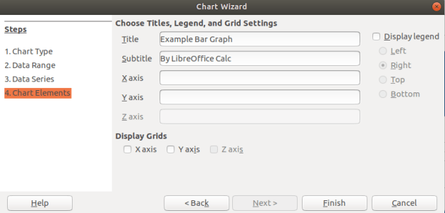
In the last window above, you can add a title and label the axes if you want. You can see that I gave my graph a name. In addition, you can decide if you want to display a legend if you look to the right. For my graph, that was not adding any additional information so I unchecked this option. When you click finish you will see the following on the spreadsheet.

Histogram
Histogram are for continuous data. Therefore, I convert my SD, D, N, A, SA to 1, 2, 3, 4, and 5. All the other steps are the same as above. The one difference is that you want to remove the spacing between bars. Below is how to do this.
Click on one of the bars in the bar graph until you see the green squares as shown below.

After you did this, there should be a new toolbar at the top of the spreadsheet. You need to click on the Green and blue cube as shown below

In the next window, you need to change the spacing to zero percent. This will change the bar graph into a histogram. Below is what the settings should look like.

When you click ok you should see the final histogram shown below

For free software this is not too bad. There are a lot of options that were left unexplained especial in regards to how you can manipulate the colors of everything and even make the plots 3D.
Conclusion
LibreOffice provides an alternative to paying for Microsoft products. The example below shows that Calc is capable of making visually appealing graphs just as Excel is.

Exploratory data analysis is the main task of a Data Scientist with as much as 60% of their time being devoted to this task. As such, the majority of their time is spent on something that is rather boring compared to building models.
This post will provide a simple example of how to analyze a dataset from the website called Kaggle. This dataset is looking at how is likely to default on their credit. The following steps will be conducted in this analysis.
This is not an exhaustive analysis but rather a simple one for demonstration purposes. The dataset is available here
Load Libraries and Data
Here are some packages we will need
import pandas as pd
import matplotlib.pyplot as plt
import seaborn as sns
from scipy.stats import norm
from sklearn import tree
from scipy import stats
from sklearn import metrics
You can load the data with the code below
df_train=pd.read_csv('/application_train.csv')
You can examine what variables are available with the code below. This is not displayed here because it is rather long
df_train.columns
df_train.head()
Missing Data
I prefer to deal with missing data first because missing values can cause errors throughout the analysis if they are not dealt with immediately. The code below calculates the percentage of missing data in each column.
total=df_train.isnull().sum().sort_values(ascending=False)
percent=(df_train.isnull().sum()/df_train.isnull().count()).sort_values(ascending=False)
missing_data=pd.concat([total,percent],axis=1,keys=['Total','Percent'])
missing_data.head()

                           Total   Percent
COMMONAREA_MEDI           214865  0.698723
COMMONAREA_AVG            214865  0.698723
COMMONAREA_MODE           214865  0.698723
NONLIVINGAPARTMENTS_MODE  213514  0.694330
NONLIVINGAPARTMENTS_MEDI  213514  0.694330
Only the first five values are printed. You can see that some variables have a large amount of missing data. As such, they are probably worthless for inclusion in additional analysis. The code below removes all variables with any missing data.
pct_null = df_train.isnull().sum() / len(df_train)
missing_features = pct_null[pct_null > 0.0].index
df_train.drop(missing_features, axis=1, inplace=True)
You can use the .head() function if you want to see how many variables are left.
Data Description & Visualization
For demonstration purposes, we will print descriptive stats and make visualizations of a few of the variables that are remaining.
round(df_train['AMT_CREDIT'].describe())
Out[8]:
count     307511.0
mean      599026.0
std       402491.0
min        45000.0
25%       270000.0
50%       513531.0
75%       808650.0
max      4050000.0

sns.distplot(df_train['AMT_CREDIT']

round(df_train['AMT_INCOME_TOTAL'].describe())
Out[10]:
count       307511.0
mean        168798.0
std         237123.0
min          25650.0
25%         112500.0
50%         147150.0
75%         202500.0
max      117000000.0
sns.distplot(df_train['AMT_INCOME_TOTAL']

I think you are getting the point. You can also look at categorical variables using the groupby() function.
We also need to address categorical variables in terms of creating dummy variables. This is so that we can develop a model in the future. Below is the code for dealing with all the categorical variables and converting them to dummy variable’s
df_train.groupby('NAME_CONTRACT_TYPE').count()
dummy=pd.get_dummies(df_train['NAME_CONTRACT_TYPE'])
df_train=pd.concat([df_train,dummy],axis=1)
df_train=df_train.drop(['NAME_CONTRACT_TYPE'],axis=1)

df_train.groupby('CODE_GENDER').count()
dummy=pd.get_dummies(df_train['CODE_GENDER'])
df_train=pd.concat([df_train,dummy],axis=1)
df_train=df_train.drop(['CODE_GENDER'],axis=1)

df_train.groupby('FLAG_OWN_CAR').count()
dummy=pd.get_dummies(df_train['FLAG_OWN_CAR'])
df_train=pd.concat([df_train,dummy],axis=1)
df_train=df_train.drop(['FLAG_OWN_CAR'],axis=1)

df_train.groupby('FLAG_OWN_REALTY').count()
dummy=pd.get_dummies(df_train['FLAG_OWN_REALTY'])
df_train=pd.concat([df_train,dummy],axis=1)
df_train=df_train.drop(['FLAG_OWN_REALTY'],axis=1)

df_train.groupby('NAME_INCOME_TYPE').count()
dummy=pd.get_dummies(df_train['NAME_INCOME_TYPE'])
df_train=pd.concat([df_train,dummy],axis=1)
df_train=df_train.drop(['NAME_INCOME_TYPE'],axis=1)

df_train.groupby('NAME_EDUCATION_TYPE').count()
dummy=pd.get_dummies(df_train['NAME_EDUCATION_TYPE'])
df_train=pd.concat([df_train,dummy],axis=1)
df_train=df_train.drop(['NAME_EDUCATION_TYPE'],axis=1)

df_train.groupby('NAME_FAMILY_STATUS').count()
dummy=pd.get_dummies(df_train['NAME_FAMILY_STATUS'])
df_train=pd.concat([df_train,dummy],axis=1)
df_train=df_train.drop(['NAME_FAMILY_STATUS'],axis=1)

df_train.groupby('NAME_HOUSING_TYPE').count()
dummy=pd.get_dummies(df_train['NAME_HOUSING_TYPE'])
df_train=pd.concat([df_train,dummy],axis=1)
df_train=df_train.drop(['NAME_HOUSING_TYPE'],axis=1)

df_train.groupby('ORGANIZATION_TYPE').count()
dummy=pd.get_dummies(df_train['ORGANIZATION_TYPE'])
df_train=pd.concat([df_train,dummy],axis=1)
df_train=df_train.drop(['ORGANIZATION_TYPE'],axis=1)
You have to be careful with this because now you have many variables that are not necessary. For every categorical variable you must remove at least one category in order for the model to work properly. Below we did this manually.
df_train=df_train.drop(['Revolving loans','F','XNA','N','Y','SK_ID_CURR,''Student','Emergency','Lower secondary','Civil marriage','Municipal apartment'],axis=1)
Below are some boxplots with the target variable and other variables in the dataset.
f,ax=plt.subplots(figsize=(8,6))
fig=sns.boxplot(x=df_train['TARGET'],y=df_train['AMT_INCOME_TOTAL'])

There is a clear outlier there. Below is another boxplot with a different variable
f,ax=plt.subplots(figsize=(8,6))
fig=sns.boxplot(x=df_train['TARGET'],y=df_train['CNT_CHILDREN'])

It appears several people have more than 10 children. This is probably a typo.
Below is a correlation matrix using a heatmap technique
corrmat=df_train.corr()
f,ax=plt.subplots(figsize=(12,9))
sns.heatmap(corrmat,vmax=.8,square=True)

The heatmap is nice but it is hard to really appreciate what is happening. The code below will sort the correlations from least to strongest, so we can remove high correlations.
c = df_train.corr().abs()

s = c.unstack()
so = s.sort_values(kind="quicksort")
print(so.head())

FLAG_DOCUMENT_12 FLAG_MOBIL 0.000005
FLAG_MOBIL FLAG_DOCUMENT_12 0.000005
Unknown FLAG_MOBIL 0.000005
FLAG_MOBIL Unknown 0.000005
Cash loans FLAG_DOCUMENT_14 0.000005
The list is to long to show here but the following variables were removed for having a high correlation with other variables.
df_train=df_train.drop(['WEEKDAY_APPR_PROCESS_START','FLAG_EMP_PHONE','REG_CITY_NOT_WORK_CITY','REGION_RATING_CLIENT','REG_REGION_NOT_WORK_REGION'],axis=1)
Below we check a few variables for homoscedasticity, linearity, and normality using plots and histograms
sns.distplot(df_train['AMT_INCOME_TOTAL'],fit=norm)
fig=plt.figure()
res=stats.probplot(df_train['AMT_INCOME_TOTAL'],plot=plt)


This is not normal
sns.distplot(df_train['AMT_CREDIT'],fit=norm)
fig=plt.figure()
res=stats.probplot(df_train['AMT_CREDIT'],plot=plt)


This is not normal either. We could do transformations, or we can make a non-linear model instead.
Model Development
Now comes the easy part. We will make a decision tree using only some variables to predict the target. In the code below we make are X and y dataset.
X=df_train[['Cash loans','DAYS_EMPLOYED','AMT_CREDIT','AMT_INCOME_TOTAL','CNT_CHILDREN','REGION_POPULATION_RELATIVE']]
y=df_train['TARGET']
The code below fits are model and makes the predictions
clf=tree.DecisionTreeClassifier(min_samples_split=20)
clf=clf.fit(X,y)
y_pred=clf.predict(X)
Below is the confusion matrix followed by the accuracy
print (pd.crosstab(y_pred,df_train['TARGET']))
TARGET       0      1
row_0
0       280873  18493
1         1813   6332
accuracy_score(y_pred,df_train['TARGET'])
Out[47]: 0.933966589813047
Lastly, we can look at the precision, recall, and f1 score
print(metrics.classification_report(y_pred,df_train['TARGET']))
              precision    recall  f1-score   support

           0       0.99      0.94      0.97    299366
           1       0.26      0.78      0.38      8145

   micro avg       0.93      0.93      0.93    307511
   macro avg       0.62      0.86      0.67    307511
weighted avg       0.97      0.93      0.95    307511
This model looks rather good in terms of accuracy of the training set. It actually impressive that we could use so few variables from such a large dataset and achieve such a high degree of accuracy.
Conclusion
Data exploration and analysis is the primary task of a data scientist. This post was just an example of how this can be approached. Of course, there are many other creative ways to do this but the simplistic nature of this analysis yielded strong results


