Category Archives: ANOVA

Kruskal-Willis Test in R

Sometimes when the data that needs to be analyzed is not normally distributed. This makes it difficult to make any inferences based on the results because one of the main assumptions of parametric statistical test such as ANOVA, t-test, etc is normal distribution of the data.

Fortunately, for every parametric test there is a non-parametric test. Non-parametric test are test that make no assumptions about the normality of the data. This means that the non-normal data can still be analyzed with a certain measure of confidence in terms of the results.

This post will look at non-parametric test that are used to test the difference in means. For three or more groups we used the Kruskal-Wallis Test. The Kruskal-Wallis Test is the non-parametric version of ANOVA.


Setup

We are going to use the “ISLR” package available on R to demonstrate the use of the Kruskal-Wallis test. After downloading this package you need to load the “Auto” data. Below is the code to do all of this.

install.packages('ISLR')
library(ISLR)
data=Auto

We now need to examine the structure of the data set. This is done with the “str” function below is code followed by the results

str(Auto)
'data.frame':	392 obs. of  9 variables:
 $ mpg         : num  18 15 18 16 17 15 14 14 14 15 ...
 $ cylinders   : num  8 8 8 8 8 8 8 8 8 8 ...
 $ displacement: num  307 350 318 304 302 429 454 440 455 390 ...
 $ horsepower  : num  130 165 150 150 140 198 220 215 225 190 ...
 $ weight      : num  3504 3693 3436 3433 3449 ...
 $ acceleration: num  12 11.5 11 12 10.5 10 9 8.5 10 8.5 ...
 $ year        : num  70 70 70 70 70 70 70 70 70 70 ...
 $ origin      : num  1 1 1 1 1 1 1 1 1 1 ...
 $ name        : Factor w/ 304 levels "amc ambassador brougham",..: 49 36 231 14 161 141 54 223 241 2 ...

So we have 9 variables. We first need to find if any of the continuous variables are non-normal because this indicates that the Kruskal-Willis test is needed. We will look at the ‘displacement’ variable and look at the histogram to see if it is normally distributed. Below is the code followed by the histogram

hist(Auto$displacement)
Rplot.jpeg

This does not look normally distributed. We now need a factor variable with 3 or more groups. We are going to use the ‘origin’ variable. This variable indicates were the care was made 1 = America, 2 = Europe, and 3 = Japan. However, this variable is currently a numeric variable. We need to change it into a factor variable. Below is the code for this

Auto$origin<-as.factor(Auto$origin)

The Test

We will now use the Kruskal-Wallis test. The question we have is “is there a difference in displacement based on the origin of the vehicle?” The code for the analysis is below followed by the results.

> kruskal.test(displacement ~ origin, data = Auto)

	Kruskal-Wallis rank sum test

data:  displacement by origin
Kruskal-Wallis chi-squared = 201.63, df = 2, p-value < 2.2e-16

Based on the results, we know there is a difference among the groups. However, just like ANOVA, we do not know were. We have to do a post-hoc test in order to determine where the difference in means is among the three groups.

To do this we need to install a new package and do a new analysis. We will download the “PCMR” package and run the code below

install.packages('PMCMR')
library(PMCMR)
data(Auto)
attach(Auto)
posthoc.kruskal.nemenyi.test(x=displacement, g=origin, dist='Tukey')

Here is what we did,

  1. Installed the PMCMR package and loaded it
  2. Loaded the “Auto” data and used the “attach” function to make it available
  3. Ran the function “posthoc.kruskal.nemenyi.test” and place the appropriate variables in their place and then indicated the type of posthoc test ‘Tukey’

Below are the results

Pairwise comparisons using Tukey and Kramer (Nemenyi) test	
                   with Tukey-Dist approximation for independent samples 

data:  displacement and origin 

  1       2   
2 3.4e-14 -   
3 < 2e-16 0.51

P value adjustment method: none 
Warning message:
In posthoc.kruskal.nemenyi.test.default(x = displacement, g = origin,  :
  Ties are present, p-values are not corrected.

The results are listed in a table. When a comparison was made between group 1 and 2 the results were significant (p < 0.0001). The same when group 1 and 3 are compared (p < 0.0001).  However, there was no difference between group 2 and 3 (p = 0.51).

Do not worry about the warning message this can be corrected if necessary

Perhaps you are wondering what the actually means for each group is. Below is the code with the results

> aggregate(Auto[, 3], list(Auto$origin), mean)
  Group.1        x
1       1 247.5122
2       2 109.6324
3       3 102.7089

Cares made in America have an average displacement of 247.51 while cars from Europe and Japan have a displacement of 109.63 and 102.70. Below is the code for the boxplot followed by the graph

boxplot(displacement~origin, data=Auto, ylab= 'Displacement', xlab='Origin')
title('Car Displacement')

Rplot01.jpeg

Conclusion

This post provided an example of the Kruskal-Willis test. This test is useful when the data is not normally distributed. The main problem with this test is that it is less powerful than an ANOVA test. However, this is a problem with most non-parametric test when compared to parametric test.

ANOVA with R

Analysis of variance (ANOVA) is used when you want to see if there is a difference in the means of three or more groups due to some form of treatment(s). In this post, we will look at conducting an ANOVA calculation using R.

We are going to use a dataset that is already built into R called ‘InsectSprays.’ This dataset contains information on different insecticides and their ability to kill insects. What we want to know is which insecticide was the best at killing insects.

In the dataset ‘InsectSprays’, there are two variables, ‘count’, which is the number of dead bugs, and ‘spray’ which is the spray that was used to kill the bug. For the ‘spray’ variable there are six types label A-F. There are 72 total observations for the six types of spray which comes to about 12 observations per spray.

Building the Model

The code for calculating the ANOVA is below

> BugModel<- aov(count ~ spray, data=InsectSprays)
> BugModel
Call:
   aov(formula = count ~ spray, data = InsectSprays)

Terms:
                   spray Residuals
Sum of Squares  2668.833  1015.167
Deg. of Freedom        5        66

Residual standard error: 3.921902
Estimated effects may be unbalanced

Here is what we did

  1. We created the variable ‘BugModel’
  2. In this variable, we used the function ‘aov’ which is the ANOVA function.
  3. Within the ‘aov’ function we told are to determine the count by the difference sprays that is what the ‘~’ tilde operator does.
  4. After the comma, we told R what dataset to use which was “InsectSprays.”
  5. Next, we pressed ‘enter’ and nothing happens. This is because we have to make R print the results by typing the name of the variable “BugModel” and pressing ‘enter’.
  6. The results do not tell us anything too useful yet. However, now that we have the ‘BugModel’ saved we can use this information to find the what we want.

Now we need to see if there are any significant results. To do this we will use the ‘summary’ function as shown in the script below

> summary(BugModel)
            Df Sum Sq Mean Sq F value Pr(>F)    
spray        5   2669   533.8    34.7 <2e-16 ***
Residuals   66   1015    15.4                   
---
Signif. codes:  0 ‘***’ 0.001 ‘**’ 0.01 ‘*’ 0.05 ‘.’ 0.1 ‘ ’ 1

These results indicate that there are significant results in the model as shown by the p-value being essentially zero (Pr(>F)). In other words, there is at least one mean that is different from the other means statistically.

We need to see what the means are overall for all sprays and for each spray individually. This is done with the following script

> model.tables(BugModel, type = 'means')
Tables of means
Grand mean
    
9.5 

 spray 
spray
     A      B      C      D      E      F 
14.500 15.333  2.083  4.917  3.500 16.667

The ‘model.tables’ function tells us the means overall and for each spray. As you can see, it appears spray F is the most efficient at killing bugs with a mean of 16.667.

However, this table does not indicate the statistically significance. For this we need to conduct a post-hoc Tukey test. This test will determine which mean is significantly different from the others. Below is the script

> BugSpraydiff<- TukeyHSD(BugModel)
> BugSpraydiff
  Tukey multiple comparisons of means
    95% family-wise confidence level

Fit: aov(formula = count ~ spray, data = InsectSprays)

$spray
           diff        lwr       upr     p adj
B-A   0.8333333  -3.866075  5.532742 0.9951810
C-A -12.4166667 -17.116075 -7.717258 0.0000000
D-A  -9.5833333 -14.282742 -4.883925 0.0000014
E-A -11.0000000 -15.699409 -6.300591 0.0000000
F-A   2.1666667  -2.532742  6.866075 0.7542147
C-B -13.2500000 -17.949409 -8.550591 0.0000000
D-B -10.4166667 -15.116075 -5.717258 0.0000002
E-B -11.8333333 -16.532742 -7.133925 0.0000000
F-B   1.3333333  -3.366075  6.032742 0.9603075
D-C   2.8333333  -1.866075  7.532742 0.4920707
E-C   1.4166667  -3.282742  6.116075 0.9488669
F-C  14.5833333   9.883925 19.282742 0.0000000
E-D  -1.4166667  -6.116075  3.282742 0.9488669
F-D  11.7500000   7.050591 16.449409 0.0000000
F-E  13.1666667   8.467258 17.866075 0.0000000

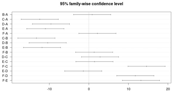
There is a lot of information here. To make things easy, wherever there is a p adj of less than 0.05 that means that there is a difference between those two means. For example, bug spray F and E have a difference of 13.16 that has a p adj of zero. So these two means are really different statistically.This chart also includes the lower and upper bounds of the confidence interval.

The results can also be plotted with the script below

> plot(BugSpraydiff, las=1)

Below is the plot

Rplot10

Conclusion

ANOVA is used to calculate if there is a difference of means among three or more groups. This analysis can be conducted in R using various scripts and codes.

Two-Way Analysis of Variance

Two-way analysis of variance is used when we want to know the following pieces of information.
• The means of the blocks or subpopulations
• The means of the treatment groups
• The means of the interaction of the subpopulation and treatment groups

Now you are probably confused but remember that two-way analysis of variance is an extension of randomized block designed. With randomized block design, there were two hypotheses one for the treatment groups and one for the blocks or subpopulations. What we are doing for two-analysis is assessing the interaction effect, which is the amount of the variation of
subpopulation and treatment group). The assessment of the interaction effect gives us the third hypothesis. To put it in simple words when both the subpopulation and the treatment are present combined they have some sort of influence just as they do when one or the other is present. Therefore, two-way analysis of variance is randomized block designed plus an interaction effect hypothesis.

Another important difference is the use of repeated measures. In a two-way analysis of variance, at least one of the groups received the treatment more than once. In a randomized block design, each group receives the treatment only one time. Your research questions determine if any group needs to experience the treatment more than once.

Below are the assumptions
• Sample randomly selected
• Populations have homogeneous standard deviations
• Population distributions are normal
• Population covariances are equal.

Here are the steps
1. Set up hypotheses (there will be three of them)
a.Treatment means (AKA factor A)
i. H0: There is no difference in the treatment means
ii. H1: H0 is false
b. Block means (AKA factor B)
i. H0: There is no difference in the block means
ii. H1: is false
c. Interaction between Factor A and B
i. H0: There is no interacting effect between factor A & B
ii. H1: There is an interacting effect between factor A & B
2. Determine your level of statistical significance
3. Determine F critical (there will be three now and the computer does this)
4. Calculate the F-test values (there will be three now and the computer does this)
5. Test hypotheses
6. State conclusion

Here is an example
A music teacher wants to study the effect of instrument type and service center on the repair time measured in minutes. Four instruments (sax, trumpet, clarinet, flute) were picked for the analysis. Each service center was assigned to perform the particular repair on two instruments in each category

Instrument
Service centers Sax Trumpet Clarinet Flute
1                        60      50          58         60
70      56          62         64
2                        50      53          48         54
54      57          64         46
3                        62      54          46         51
64      66          52         49

Here are your research questions
• Is there a difference in the means of the repair time between service centers?
• Is there a difference in the means of the repair time between instrument type?
• Is there an interaction due to service center and type of instrument on the mean of the repair time
Let us go through each of our steps
Step 1: State the hypotheses
• Treatment means (AKA factor A)
a. H0: There is no difference in the means of the service centers
b. H1: H0 is false
• Block means (AKA factor B)
a. H0: There is no difference in means of the instrument types
b. H1: is false
• Interaction between Factor A and B
a. H0: There is no interacting effect between service center and instrument type
b. H1: There is an interacting effect between service center and instrument type

Step 2: Significance level
• Set at 0.1

Step 3: Determine F-Critical
For the instruments, F-critical is 2.81
For the service centers, F-critical is 2.61
For the interaction effect, F-critical is 2.33

Step 4: Calculate F-values
Service centers 3.2
Instrument type 1.4
Interaction 2.1

Step 5: Make decision
Since the F-value of 3.2 is greater than the F-critical of 2.8 we reject the null hypothesis for the service centers

Since the F-value of 1.4 is less than the F-critical of 2.61 we do not reject the null hypothesis for the instrument types

Since the F-value of 2.1 is less than the F-critical of 2.3 we do reject the null hypothesis for the interaction effect of service center and instrument type.

Step 6: Conclusion
Since we reject the null hypothesis that there is no difference in the means of the repair time of the service centers, we conclude that there is evidence of a difference in the repair times between service centers. This means that one service center is faster than the others are. To find out, do a posthoc test.

Since we do not reject the null hypothesis that there is no difference in the means of the repair time of the instrument types, we conclude that there is no evidence of a difference in the repair time between instrument types. In other words, it does not matter what type of instrument is being fixed as they will all take about the same amount of time.

Since we do not reject the null hypothesis that there is no interaction effect of service center and instrument type on the mean of the repair time, we conclude that there is no evidence of an interaction effect of service center and instrument type on repair time. In other words, if service center and instrument type are considered at the same time there is no difference in how fast the instruments are repaired.

Analysis of Variance: Randomized Block Design

Randomized blocked design is used when a researcher wants to compare treatment means. What is unique to this research design is that the experiment is divided into two or more mini-experiments.

The reason behind this is to reduce the variation within-treatments so that it is easier to find differences between means.  Another unique characteristic of randomized block design is that since there is more than one experiment happening at the same time, there will be more than one set of hypotheses to consider. There will be a set of hypotheses for the treatment groups and also for the block groups. The block groups are the several subpopulations with the sample. Below are the assumptions

  • Samples are randomly selected
  • Populations are homogeneous
  • Populations are normally distributed
  • Populations covariances are equal
    •  Covariance is a measure of the commonality that two variables deviate from their expected values. If two variable deviates in similar ways the covariance will be high and vice versa. The standardized version of covariance is correlation.

Looking at equations and doing this by hand is tough. It is better to use SPSS or excel to calculate results. We are going to look at an example and see an application of randomized block design.

A professor wants to see if “time of day” affects his students score on a quiz. He randomly divides his stat class into five groups and has them take the quiz at one of four times during the day.  Below are the results
Time Period/Treatment
Section    8-9                10-11                11-12                1-2
1                  25                      22                        20                     25
2                  28                      24                        29                     23
3                  30                      25                        25                     27
4                  24                      27                        28                     25
5                  21                      28                        30                     24

The treatment groups here are the time periods. The are along the time and are 8-9, 10-11, 11-12, 1-2. The block groups are along the left-hand side and the are section 1, 2, 3, 4, 5. The block groups are the 5 different experimental groups of the larger population of the statistics class. What is happening here is that all members from all groups all took the quiz at one of the four times. For example, members from section one took the quiz at 8-9, 10-11, 11-12, and 1-2. The same for group 2 and so forth.  By having five different groups take the quiz at each of the time periods it should hopefully improve the accuracy of the results. It is like sampling a population five times instead of one time.

In addition, by having four different time periods, we can hopefully see much more clearly if the time period makes a difference. We have four different time periods instead of two or three. Below are the steps for solving this problem.

Step 1: State hypotheses
For Time periods
Null hypothesis: There is no difference in the means between time periods
Alternative hypothesis: There is a difference in the means between time periods
For Blocks
Null hypothesis: There is no difference in the means among the sections of students
Alternative hypothesis: There is difference in the means among the sections of students

Step 2: Significance level
are alpha is set to .05

Step 3: Critical value of F
This is done by the computer and it indicates that the F critical for the treatment (time periods) is 3.49 and the F critical for the blocks (section of students) is 3.26. There are two F criticals because there are two sets of hypotheses, one for the time periods and one for the students.

Step 4: Calculate
The computed F-value for treatment (time periods) is 0.25
The computed F-value for the blocks (section of students) is 0.89

Step 5: Decision
Since the F-value of the treatment (time periods) is 0.25 is less than F critical of 3.49 at an alpha of .05 we do not reject the null hypothesis

Since the F-value of the blocks (section of students) is 0.89 is less than F critical of 3.26 at an alpha of .05 we do not reject the null hypothesis

Step 6: Conclusion
Treatment (Time period)
Since we did not reject the null hypothesis, we can conclude that there is no evidence that time of day affects the quiz scores.

Blocks (Section of Student)
Since we did not reject the null hypothesis, we can conclude that there is no evidence that group affects the quiz scores.

From this, we know that time of day and the group a student belongs to does not matter. If the time of day mattered it might have been due to a host of factors such as early morning or late afternoon. For the groups, the difference could be identified by how they did on individual items. Maybe they struggled with finding the means of question 3.

Remember in this example there was no difference. The ideas above are for determining why there was a difference if that had happened.

One-Way Analysis of Variance (ANOVA)

Analysis of variance is a statistical technique that is used to determine if there is a difference in two or more sample populations.  Z-test and t-tests are used when comparing one sample population to a known value or two sample populations to each other. When two or more sample populations are involved it is necessary to use analysis of variance.  The simple rule is 3 or more use analysis of variance

Analysis of variance is too complicated to do by hand, even though it is possible. It takes a great deal of time and one error will ruin the answer. Therefore, we are not going to look at equations during this example. Instead, we will focus on the hypotheses and practical applications of analysis of variance. To calculate analysis of variance results you can use SPSS or Microsoft excel.

There are several types of analysis of variance. We are going to first look at one-way analysis of variance.

Here are the assumptions for one-way analysis of variance

  • Samples are randomly selected
  • Samples are independently assigned
  • Samples are homogeneous
  • Sample is normally distributed

One-way analysis of variance is used when 2 or more groups receive the same treatment or intervention. The treatment is the independent variable while the means of each group is the dependent variable. This is because as the researcher, you control the treatment but you do not control the resulting mean that is recorded. One-way analysis of variance is often used in performing experiments.

Let’s look at an example. You want to know if there is any difference in the average life of four different breeds of dogs. You take a random sample of five dogs from four different breeds. Below are the results

Terrier    Retriever   Hound   Bulldog
12                 11                   12            12
13                 10                   11             15
14                 13                   15             10
11                 15                   15             12
15                 14                   16             11

In this example, the independent variable is the breed of dog. This is because you control this. You can select whatever dog breed you want. The dependent variable is the average length of the dog’s lives. You have no control over how long they live. You are trying to see if  dog breed influences how long the dog will live

Here are the hypotheses

Null hypotheses: There is no difference in the average length of a dog’s life because of breed

Alternative hypotheses: There is a difference in the average length of a dog’s life because of breed

The significance level is 0.05  are F critical is 3.24

After running the results in the computer we get an F-value of 0.76. This means we do not reject are null hypotheses.  This means that there is no difference in the average life of the dog breeds in this study.

One-way analysis is used when we have one treatment and three or more groups that experience the treatment. This statistical tool is useful for research designs that call on the need for experiments.