Analysis of variance (ANOVA) is used when you want to see if there is a difference in the means of three or more groups due to some form of treatment(s). In this post, we will look at conducting an ANOVA calculation using R.

We are going to use a dataset that is already built into R called ‘InsectSprays.’ This dataset contains information on different insecticides and their ability to kill insects. What we want to know is which insecticide was the best at killing insects.

In the dataset ‘InsectSprays’, there are two variables, ‘count’, which is the number of dead bugs, and ‘spray’ which is the spray that was used to kill the bug. For the ‘spray’ variable there are six types label A-F. There are 72 total observations for the six types of spray which comes to about 12 observations per spray.

Building the Model

The code for calculating the ANOVA is below

> BugModel<- aov(count ~ spray, data=InsectSprays)
> BugModel
Call:
   aov(formula = count ~ spray, data = InsectSprays)

Terms:
                   spray Residuals
Sum of Squares  2668.833  1015.167
Deg. of Freedom        5        66

Residual standard error: 3.921902
Estimated effects may be unbalanced

Here is what we did

1. We created the variable ‘BugModel’
2. In this variable, we used the function ‘aov’ which is the ANOVA function.
3. Within the ‘aov’ function we told are to determine the count by the difference sprays that is what the ‘~’ tilde operator does.
4. After the comma, we told R what dataset to use which was “InsectSprays.”
5. Next, we pressed ‘enter’ and nothing happens. This is because we have to make R print the results by typing the name of the variable “BugModel” and pressing ‘enter’.
6. The results do not tell us anything too useful yet. However, now that we have the ‘BugModel’ saved we can use this information to find the what we want.

Now we need to see if there are any significant results. To do this we will use the ‘summary’ function as shown in the script below

> summary(BugModel)
            Df Sum Sq Mean Sq F value Pr(>F)    
spray        5   2669   533.8    34.7 <2e-16 ***
Residuals   66   1015    15.4                   
---
Signif. codes:  0 ‘***’ 0.001 ‘**’ 0.01 ‘*’ 0.05 ‘.’ 0.1 ‘ ’ 1

These results indicate that there are significant results in the model as shown by the p-value being essentially zero (Pr(>F)). In other words, there is at least one mean that is different from the other means statistically.

We need to see what the means are overall for all sprays and for each spray individually. This is done with the following script

> model.tables(BugModel, type = 'means')
Tables of means
Grand mean
    
9.5 

 spray 
spray
     A      B      C      D      E      F 
14.500 15.333  2.083  4.917  3.500 16.667

The ‘model.tables’ function tells us the means overall and for each spray. As you can see, it appears spray F is the most efficient at killing bugs with a mean of 16.667.

However, this table does not indicate the statistically significance. For this we need to conduct a post-hoc Tukey test. This test will determine which mean is significantly different from the others. Below is the script

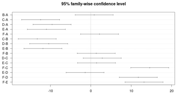
> BugSpraydiff<- TukeyHSD(BugModel)
> BugSpraydiff
  Tukey multiple comparisons of means
    95% family-wise confidence level

Fit: aov(formula = count ~ spray, data = InsectSprays)

$spray
           diff        lwr       upr     p adj
B-A   0.8333333  -3.866075  5.532742 0.9951810
C-A -12.4166667 -17.116075 -7.717258 0.0000000
D-A  -9.5833333 -14.282742 -4.883925 0.0000014
E-A -11.0000000 -15.699409 -6.300591 0.0000000
F-A   2.1666667  -2.532742  6.866075 0.7542147
C-B -13.2500000 -17.949409 -8.550591 0.0000000
D-B -10.4166667 -15.116075 -5.717258 0.0000002
E-B -11.8333333 -16.532742 -7.133925 0.0000000
F-B   1.3333333  -3.366075  6.032742 0.9603075
D-C   2.8333333  -1.866075  7.532742 0.4920707
E-C   1.4166667  -3.282742  6.116075 0.9488669
F-C  14.5833333   9.883925 19.282742 0.0000000
E-D  -1.4166667  -6.116075  3.282742 0.9488669
F-D  11.7500000   7.050591 16.449409 0.0000000
F-E  13.1666667   8.467258 17.866075 0.0000000

There is a lot of information here. To make things easy, wherever there is a p adj of less than 0.05 that means that there is a difference between those two means. For example, bug spray F and E have a difference of 13.16 that has a p adj of zero. So these two means are really different statistically.This chart also includes the lower and upper bounds of the confidence interval.

The results can also be plotted with the script below

> plot(BugSpraydiff, las=1)

Below is the plot

Conclusion

ANOVA is used to calculate if there is a difference of means among three or more groups. This analysis can be conducted in R using various scripts and codes.