Category Archives: R programming

Kruskal-Willis Test in R

Sometimes when the data that needs to be analyzed is not normally distributed. This makes it difficult to make any inferences based on the results because one of the main assumptions of parametric statistical test such as ANOVA, t-test, etc is normal distribution of the data.

Fortunately, for every parametric test there is a non-parametric test. Non-parametric test are test that make no assumptions about the normality of the data. This means that the non-normal data can still be analyzed with a certain measure of confidence in terms of the results.

This post will look at non-parametric test that are used to test the difference in means. For three or more groups we used the Kruskal-Wallis Test. The Kruskal-Wallis Test is the non-parametric version of ANOVA.


Setup

We are going to use the “ISLR” package available on R to demonstrate the use of the Kruskal-Wallis test. After downloading this package you need to load the “Auto” data. Below is the code to do all of this.

install.packages('ISLR')
library(ISLR)
data=Auto

We now need to examine the structure of the data set. This is done with the “str” function below is code followed by the results

str(Auto)
'data.frame':	392 obs. of  9 variables:
 $ mpg         : num  18 15 18 16 17 15 14 14 14 15 ...
 $ cylinders   : num  8 8 8 8 8 8 8 8 8 8 ...
 $ displacement: num  307 350 318 304 302 429 454 440 455 390 ...
 $ horsepower  : num  130 165 150 150 140 198 220 215 225 190 ...
 $ weight      : num  3504 3693 3436 3433 3449 ...
 $ acceleration: num  12 11.5 11 12 10.5 10 9 8.5 10 8.5 ...
 $ year        : num  70 70 70 70 70 70 70 70 70 70 ...
 $ origin      : num  1 1 1 1 1 1 1 1 1 1 ...
 $ name        : Factor w/ 304 levels "amc ambassador brougham",..: 49 36 231 14 161 141 54 223 241 2 ...

So we have 9 variables. We first need to find if any of the continuous variables are non-normal because this indicates that the Kruskal-Willis test is needed. We will look at the ‘displacement’ variable and look at the histogram to see if it is normally distributed. Below is the code followed by the histogram

hist(Auto$displacement)
Rplot.jpeg

This does not look normally distributed. We now need a factor variable with 3 or more groups. We are going to use the ‘origin’ variable. This variable indicates were the care was made 1 = America, 2 = Europe, and 3 = Japan. However, this variable is currently a numeric variable. We need to change it into a factor variable. Below is the code for this

Auto$origin<-as.factor(Auto$origin)

The Test

We will now use the Kruskal-Wallis test. The question we have is “is there a difference in displacement based on the origin of the vehicle?” The code for the analysis is below followed by the results.

> kruskal.test(displacement ~ origin, data = Auto)

	Kruskal-Wallis rank sum test

data:  displacement by origin
Kruskal-Wallis chi-squared = 201.63, df = 2, p-value < 2.2e-16

Based on the results, we know there is a difference among the groups. However, just like ANOVA, we do not know were. We have to do a post-hoc test in order to determine where the difference in means is among the three groups.

To do this we need to install a new package and do a new analysis. We will download the “PCMR” package and run the code below

install.packages('PMCMR')
library(PMCMR)
data(Auto)
attach(Auto)
posthoc.kruskal.nemenyi.test(x=displacement, g=origin, dist='Tukey')

Here is what we did,

  1. Installed the PMCMR package and loaded it
  2. Loaded the “Auto” data and used the “attach” function to make it available
  3. Ran the function “posthoc.kruskal.nemenyi.test” and place the appropriate variables in their place and then indicated the type of posthoc test ‘Tukey’

Below are the results

Pairwise comparisons using Tukey and Kramer (Nemenyi) test	
                   with Tukey-Dist approximation for independent samples 

data:  displacement and origin 

  1       2   
2 3.4e-14 -   
3 < 2e-16 0.51

P value adjustment method: none 
Warning message:
In posthoc.kruskal.nemenyi.test.default(x = displacement, g = origin,  :
  Ties are present, p-values are not corrected.

The results are listed in a table. When a comparison was made between group 1 and 2 the results were significant (p < 0.0001). The same when group 1 and 3 are compared (p < 0.0001).  However, there was no difference between group 2 and 3 (p = 0.51).

Do not worry about the warning message this can be corrected if necessary

Perhaps you are wondering what the actually means for each group is. Below is the code with the results

> aggregate(Auto[, 3], list(Auto$origin), mean)
  Group.1        x
1       1 247.5122
2       2 109.6324
3       3 102.7089

Cares made in America have an average displacement of 247.51 while cars from Europe and Japan have a displacement of 109.63 and 102.70. Below is the code for the boxplot followed by the graph

boxplot(displacement~origin, data=Auto, ylab= 'Displacement', xlab='Origin')
title('Car Displacement')

Rplot01.jpeg

Conclusion

This post provided an example of the Kruskal-Willis test. This test is useful when the data is not normally distributed. The main problem with this test is that it is less powerful than an ANOVA test. However, this is a problem with most non-parametric test when compared to parametric test.

Decisions Trees with Titanic

In this post, we will make predictions about Titanic survivors using decision trees. The advantage of decisions trees is that they split the data into clearly defined groups. This process continues until the data is divided into extremely small subsets. This subsetting is used for making predictions.

We are assuming you have the data and have viewed the previous machine learning post on this blog. If not please click here.

Beginnings

You need to install the ‘rpart’ package from the CRAN repository as the package contains a decision tree function.You will also need to install the following packages

  • ratttle
  • rpart.plot
  • RColorNrewer

Each of these packages plays a role in developing decision trees

Building the Model

Once you have installed the packages. You need to develop the model below is the code. The model uses most of the variables in the data set for predicting survivors.

tree <- rpart(Survived~Pclass+Sex+Age+SibSp+Parch+Fare+Embarked,data=train, method=’class’)

The ‘rpart’ function is used for making the classification tree aka decision tree.

We now need to see the tree we do this with the code below

plot(tree)
text(tree)

Plot makes the tree and ‘text’ adds names download

You can probably tell that this is an ugly plot. To improve the appearance we will run the following code.

library(rattle)
library(rpart.plot)
library(RColorBrewer)
fancyRpartPlot(my_tree_two)

Below is the revised plot

download

This looks much better

How to Read

Here is one way to read a decision tree.

  1. At the top node, keep in mind we are predicting Survival rate. There is a 0 or 1 in all of the ‘buckets’. This number represents how the bucket voted. If more than 50% perish than the bucket votes ‘0’ or no survivors
  2. Still looking at the top bucket, 62% of the passengers die while 38% survived before we even split the data.The number under the node tells what percentage of the sample is in this “bucket”. For the first bucket 100% of the sample is represented.
  3. The first split is based on sex. If the person is male you look to the left. For males, 81% of them died compared to 19% who survived and the bucket votes 0 for death. 65% of the sample is in this bucket
  4. For those who are not male (female) we look to the right and see that only 26% died compared to 74% who survived leading to this bucket voting 1 for survival. This bucket represents 35% of the entire sample.
  5. This process continues all the way down to the bottom

Conclusion

Decisions trees are useful for making ‘decisions’ about what is happening in data. For those who are looking for a simple prediction algorithm, decision trees is one place to begin

Data Science Application: Titanic Survivors

This post will provide a practical application of some of the basics of data science using data from the sinking of the Titanic. In this post, in particular, we will explore the dataset and see what we can uncover.

Loading the Dataset

The first thing that we need to do is load the actual datasets into R. In machine learning, there are always at least two datasets. One dataset is the training dataset and the second dataset is the testing dataset. The training is used for developing a model and the testing is used for checking the accuracy of the model on a different dataset. Downloading both datasets can be done through the use of the following code.

url_train <- "http://s3.amazonaws.com/assets.datacamp.com/course/Kaggle/train.csv"
url_test <- "http://s3.amazonaws.com/assets.datacamp.com/course/Kaggle/test.csv"
training <- read.csv(url_train)
testing <- read.csv(url_test)

What Happen?

  1. We created the variable “url_train” and put the web link in quotes. We then repeat this for the test data set
  2. Next, we create the variable “training” and use the function “read.csv” for our “url_train” variable. This tells R to read the csv file at the web address in ‘url_train’. We then repeat this process for the testing variable

Exploration

We will now do some basic data exploration. This will help us to see what is happening in the data. What to look for is endless. Therefore, we will look at a few basics things that we might need to know. Below are some questions with answers.

  1. What variables are in the dataset?

This can be found by using the code below

str(training)

The output reveals 12 variables

'data.frame':	891 obs. of  12 variables:
 $ PassengerId: int  1 2 3 4 5 6 7 8 9 10 ...
 $ Survived   : int  0 1 1 1 0 0 0 0 1 1 ...
 $ Pclass     : int  3 1 3 1 3 3 1 3 3 2 ...
 $ Name       : Factor w/ 891 levels "Abbing, Mr. Anthony",..: 109 191 354 273 16 555 516 625 413 577 ...
 $ Sex        : Factor w/ 2 levels "female","male": 2 1 1 1 2 2 2 2 1 1 ...
 $ Age        : num  22 38 26 35 35 NA 54 2 27 14 ...
 $ SibSp      : int  1 1 0 1 0 0 0 3 0 1 ...
 $ Parch      : int  0 0 0 0 0 0 0 1 2 0 ...
 $ Ticket     : Factor w/ 681 levels "110152","110413",..: 524 597 670 50 473 276 86 396 345 133 ...
 $ Fare       : num  7.25 71.28 7.92 53.1 8.05 ...
 $ Cabin      : Factor w/ 148 levels "","A10","A14",..: 1 83 1 57 1 1 131 1 1 1 ...
 $ Embarked   : Factor w/ 4 levels "","C","Q","S": 4 2 4 4 4 3 4 4 4 2 ...

Here is a better explanation of each

  • PassengerID-ID number of each passenger
  • Survived-Who survived as indicated by a 1 and who did not by a 0
  • Pclass-Class of passenger 1st class, 2nd class, 3rd class
  • Name-The full name of a passenger
  • Sex-Male or female
  • Age-How old a passenger was
  • SibSp-Number of siblings and spouse a passenger had on board
  • Parch-Number of parents and or children a passenger had
  • Ticket-Ticket number
  • Fare-How much a ticket cost a passenger
  • Cabin-Where they slept on the titanic
  • Embarked-What port they came from

2. How many people survived in the training data?

The answer for this is found by running the following code in the R console. Keep in mind that 0 means died and 1 means survived

> table(training$Survived)
  0   1 
549 342

Unfortunately, unless you are really good at math these numbers do not provide much context. It is better to examine this using percentages as can be found in the code below.

> prop.table(table(training$Survived))

        0         1 
0.6161616 0.3838384 

These results indicate that about 62% of the passengers died while 38% survived in the training data.

3. What percentage of men and women survived?

This information can help us to determine how to setup a model for predicting who will survive. The answer is below. This time we only look percentages.

> prop.table(table(training$Sex, training$Survived), 1)
        
                 0         1
  female 0.2579618 0.7420382
  male   0.8110919 0.1889081

You can see that being male was not good on the titanic. Men died in much higher proportions compared to women.

4. Who survived by class?

The code for this is below

> prop.table(table(train$Pclass, train$Survived), 1)
   
            0         1
  1 0.3703704 0.6296296
  2 0.5271739 0.4728261
  3 0.7576375 0.2423625

Here is a code for a plot of this information followed by the plot

plot(deathbyclass, main="Passenger Fate by Traveling Class", shade=FALSE, 
+      color=TRUE, xlab="Pclass", ylab="Survived")
Rplot

3rd class had the highest mortality rate. This makes sense as 3rd class was the cheapest tickets.

5. Does age make a difference in survival?

We want to see if age matters in survival. It would make sense that younger people would be more likely to survive. This might be due to parents give their kids a seat on the lifeboats and younger singles pushing their way past older people.

We cannot use a plot for this because we would have several dozen columns on the x-axis for each year of life. Instead, we will use a box plot based on survived or died to see. Below is the code followed by a visual.

boxplot(training$Age ~ training$Survived, 
        main="Passenger Fate by Age",
        xlab="Survived", ylab="Age")

Rplot01

As you can see, there is little difference in terms of who survives based on age. This means that age may not be a useful predictor of survival.

Conclusion

Here is what we know so far

  • Sex makes a major difference in survival
  • Class makes a major difference in survival
  • Age may not make a difference in survival

There is so much more we can explore in the data. However, this is enough for beginning to lay down criteria for developing a model.

Big Data & Data Mining

Dealing with large amounts of data has been a problem throughout most of human history. Ancient civilizations had to keep large amounts of clay tablets, papyrus, steles, parchments, scrolls etc. to keep track of all the details of an empire.

However, whenever it seemed as though there would be no way to hold any more information a new technology would be developed to alleviate the problem. When people could not handle keeping records on stone paper scrolls were invented. When scrolls were no longer practical books were developed. When hand-copying books were too much the printing press came along.

By the mid 20th century there were concerns that we would not be able to have libraries large enough to keep all of the books that were being developed. With this problem came the solution of the computer. One computer could hold the information of several dozen if not hundreds of libraries.

Now even a single computer can no longer cope with all of the information that is constantly being developed for just a single subject. This has lead to computers working together in networks to share the task of storing information. With data spread across several computers, it makes analyzing data much more challenging. It was now necessary to mine for useful information in a way that people used to mine for gold in the 19th century.

Big data is data that is too large to fit within the memory of a single computer. Analyzing data that is spread across a network of databases takes skills different from traditional statistical analysis. This post will explain some of the characteristics of big data as well as data mining.

Big Data Traits

The three main traits of big data are volume, velocity, and variety. Volume describes the size of big data, which means data to big to be on only one computer. Velocity is about how fast the data can be processed. Lastly, variety different types of data. common sources of big data includes the following

  • Metadata from visual sources such as cameras
  • Data from sensors such as in medical equipment
  • Social media data such as information from google, youtube or facebook

Data Mining

Data mining is the process of discovering a model in a big dataset. Through the development of an algorithm, we can find specific information that helps us to answer our questions. Generally, there are two ways to mine data and these are extraction and summarization.

Extraction is the process of pulling specific information from a big dataset. For example, if we want all the addresses of people who bought a specific book from Amazon the result would be an extraction from a big data set.

Summarization is reducing a dataset to describe it. We might do a cluster analysis in which similar data is combined on a characteristic. For example, if we analyze all the books people ordered through Amazon last year we might notice that one cluster of groups buys mostly religious books while another buys investment books.

Conclusion

Big data will only continue to get bigger. Currently, the response has been to just use more computers and servers. As such, there is now a need for finding information on many computers and servers. This is the purpose of data mining, which is to find pertinent information that answers stakeholders questions.

Boosting in R

Boosting is a technique used to sort through many predictors in order to find the strongest through weighing them. In order to do this, you tell R to use a specific classifier such as a tree or regression model. R than makes multiple models or trees while trying to reduce the error in each model as much as possible. The weight of each predictor is based on the amount of error it reduces as an average across the models.

We will now go through an example of boosting use the “College” dataset from the “ISLR” package.

Load Packages and Setup Training/Testing Sets

First, we will load the required packages and create the needed datasets. Below is the code for this.

library(ISLR); data("College");library(ggplot2);
library(caret)
intrain<-createDataPartition(y=College$Grad.Rate, p=0.7,
 list=FALSE)
trainingset<-College[intrain, ]; testingset<-
 College[-intrain, ]

Develop the Model

We will now create the model. We are going to use all of the variables in the dataset for this example to predict graduation rate. To use all available variables requires the use of the “.” symbol instead of listing every variable name in the model. Below is the code.

Model <- train(Grad.Rate ~., method='gbm', 
 data=trainingset, verbose=FALSE)

The method we used is ‘gbm’ which stands for boosting with trees. This means that we are using the boosting feature for making decision trees.

Once the model is created you can check the results by using the following code

summary(Model)

The output is as follows (for the first 5 variables only).

                    var    rel.inf
Outstate       Outstate 36.1745640
perc.alumni perc.alumni 14.0532312
Top25perc     Top25perc 13.0194117
Apps               Apps  5.7415103
F.Undergrad F.Undergrad  5.7016602

These results tell you what the most influential variables are in predicting graduation rate. The strongest predictor was “Outstate”. This means that as the number of outstate students increases it leads to an increase in the graduation rate. You can check this by running a correlation test between ‘Outstate’ and ‘Grad.Rate’.

The next two variables are the percentage of alumni and top 25 percent. The more alumni the higher the grad rate and the more people in the top 25% the higher the grad rate.

A Visual

We will now make plot comparing the predicted grad rate with the actual grade rate. Below is the code followed by the plot.

qplot(predict(Model, testingset), Grad.Rate, data = testingset)

Rplot10

The model looks sound based on the visual inspection.

Conclusion

Boosting is a useful way to found out which predictors are strongest. It is an excellent way to explore a model to determine this for future processing.

Random Forest in R

Random Forest is a similar machine learning approach to decision trees. The main difference is that with random forest. At each node in the tree, the variable is bootstrapped. In addition, several different trees are made and the average of the trees are presented as the results. This means that there is no individual tree to analyze but rather a ‘forest’ of trees

The primary advantage of random forest is accuracy and prevent overfitting. In this post, we will look at an application of random forest in R. We will use the ‘College’ data from the ‘ISLR’ package to predict whether a college is public or private

Preparing the Data

First, we need to split our data into a training and testing set as well as load the various packages that we need. We have run this code several times when using machine learning. Below is the code to complete this.

library(ggplot2);library(ISLR)
library(caret)
data("College")
forTrain<-createDataPartition(y=College$Private, p=0.7, list=FALSE)
trainingset<-College[forTrain, ]
testingset<-College[-forTrain, ]

Develop the Model

Next, we need to setup the model we want to run using Random Forest. The coding is similar to that which is used for regression. Below is the code

Model1<-train(Private~Grad.Rate+Outstate+Room.Board+Books+PhD+S.F.Ratio+Expend, data=trainingset, method='rf',prox=TRUE)

We are using 7 variables to predict whether a university is private or not. The method is ‘rf’ which stands for “Random Forest”. By now, I am assuming you can read code and understand what the model is trying to do. For a refresher on reading code for a model please click here.

Reading the Output

If you type “Model1” followed by pressing enter, you will receive the output for the random forest

Random Forest 

545 samples
 17 predictors
  2 classes: 'No', 'Yes' 

No pre-processing
Resampling: Bootstrapped (25 reps) 
Summary of sample sizes: 545, 545, 545, 545, 545, 545, ... 
Resampling results across tuning parameters:

  mtry  Accuracy   Kappa      Accuracy SD  Kappa SD  
  2     0.8957658  0.7272629  0.01458794   0.03874834
  4     0.8969672  0.7320475  0.01394062   0.04050297
  7     0.8937115  0.7248174  0.01536274   0.04135164

Accuracy was used to select the optimal model using 
 the largest value.
The final value used for the model was mtry = 4.

Most of this is self-explanatory. The main focus is on the mtry, accuracy, and Kappa.

The shows several different models that the computer generated. Each model reports the accuracy of the model as well as the Kappa. The accuracy states how well the model predicted accurately whether a university was public or private. The kappa shares the same information but it calculates how well a model predicted while taking into account chance or luck. As such, the Kappa should be lower than the accuracy.

At the bottom of the output, the computer tells which mtry was the best. For our example, the best mtry was number 4. If you look closely, you will see that mtry 4 had the highest accuracy and Kappa as well.

Confusion Matrix for the Training Data

Below is the confusion matrix for the training data using the model developed by the random forest. As you can see, the results are different from the random forest output. This is because this model is predicting without bootstrapping

> predNew<-predict(Model1, trainingset) > trainingset$predRight<-predNew==trainingset$Private > table(predNew, trainingset$Private)
       
predNew  No Yes
    No  149   0
    Yes   0 396

Results of the Testing Data

We will now use the testing data to check the accuracy of the model we developed on the training data. Below is the code followed by the output

pred <- predict(Model1, testingset)
testingset$predRight<-pred==testingset$Private
table(pred, testingset$Private)
pred   No Yes
  No   48  11
  Yes  15 158

For the most part, the model we developed to predict if a university is private or not is accurate.

How Important is a Variable

You can calculate how important an individual variable is in the model by using the following code

Model1RF<-randomForest(Private~Grad.Rate+Outstate+Room.Board+Books+PhD+S.F.Ratio+Expend, data=trainingset, importance=TRUE)
importance(Model1RF)

The output tells you how much the accuracy of the model is reduced if you remove the variable. As such, the higher the number the more valuable the variable is in improving accuracy.

Conclusion

This post exposed you to the basics of random forest. Random forest is a technique that develops a forest of decisions trees through resampling. The results of all these trees are then averaged to give you an idea of which variables are most useful in prediction.

Decision Trees in R

Decision trees are useful for splitting data based into smaller distinct groups based on criteria you establish. This post will attempt to explain how to develop decision trees in R.

We are going to use the ‘College’ dataset found in the “ISLR” package. Once you load the package you need to split the data into a training and testing set as shown in the code below. We want to divide the data based on education level, age, and income
library(ISLR); library(ggplot2); library(caret)
data("College")
inTrain<-createDataPartition(y=College$education, 
 p=0.7, list=FALSE)
trainingset <- College[inTrain, ]
testingset <- College[-inTrain, ]

Visualize the Data

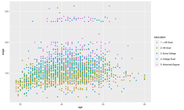
We will now make a plot of the data based on education as the groups and age and wage as the x and y variable. Below is the code followed by the plot. Please note that education is divided into 5 groups as indicated in the chart.

qplot(age, wage, colour=education, data=trainingset)
Rplot10
Create the Model

We are now going to develop the model for the decision tree. We will use age and wage to predict education as shown in the code below.

TreeModel<-train(education~age+income, method='rpart', data=trainingset)

Create Visual of the Model

We now need to create a visual of the model. This involves installing the package called ‘rattle’. You can install ‘rattle’ separately yourself. After doing this below is the code for the tree model followed by the diagram.

fancyRpartPlot(TreeModel$finalModel)

Rplot02

Here is what the chart means

  1. At the top is node 1 which is called ‘HS Grad” the decimals underneath is the percentage of the data that falls within the “HS Grad” category. As the highest node, everything is classified as “HS grad” until we begin to apply our criteria.
  2. Underneath nod 1 is a decision about wage. If a person makes less than 112 you go to the left if they make more you go to the right.
  3. Nod 2 indicates the percentage of the sample that was classified as HS grade regardless of education. 14% of those with less than a HS diploma were classified as a HS Grade based on wage. 43% of those with a HS diploma were classified as a HS grade based on income. The percentage underneath the decimals indicates the total amount of the sample placed in the HS grad category. Which was 57%.
  4. This process is repeated for each node until the data is divided as much as possible.

Predict

You can predict individual values in the dataset by using the ‘predict’ function with the test data as shown in the code below.

predict(TreeModel, newdata = testingset)

Conclusion

Prediction Trees are a unique feature in data analysis for determining how well data can be divided into subsets. It also provides a visual of how to move through data sequentially based on characteristics in the data.

Multiple Regression Prediction in R

In this post, we will learn how to predict using multiple regression in R. In a previous post, we learn how to predict with simple regression. This post will be a large repeat of this other post with the addition of using more than one predictor variable. We will use the “College” dataset and we will try to predict Graduation rate with the following variables
  • Student to faculty ratio
  • Percentage of faculty with PhD
  • Expenditures per student

Preparing the Data

First we need to load several packages and divide the dataset int training and testing sets. This is not new for this blog. Below is the code for this.

library(ISLR); library(ggplot2); library(caret)
data("College")
inTrain<-createDataPartition(y=College$Grad.Rate, 
 p=0.7, list=FALSE)
trainingset <- College[inTrain, ]
testingset <- College[-inTrain, ]
dim(trainingset); dim(testingset)

Visualizing the Data

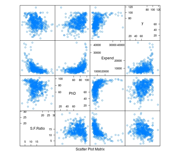
We now need to get a visual idea of the data. Since we are using several variables the code for this is slightly different so we can look at several charts at the same time. Below is the code followed by the plots

> featurePlot(x=trainingset[,c("S.F.Ratio","PhD","Expend")],y=trainingset$Grad.Rate, plot="pairs")
Rplot10

To make these plots we did the following

  1. We used the ‘featureplot’ function told R to use the ‘trainingset’ data set and subsetted the data to use the three independent variables.
  2. Next, we told R what the y= variable was and told R to plot the data in pairs

Developing the Model

We will now develop the model. Below is the code for creating the model. How to interpret this information is in another post.

> TrainingModel <-lm(Grad.Rate ~ S.F.Ratio+PhD+Expend, data=trainingset) > summary(TrainingModel)

As you look at the summary, you can see that all of our variables are significant and that the current model explains 18% of the variance of graduation rate.

Visualizing the Multiple Regression Model

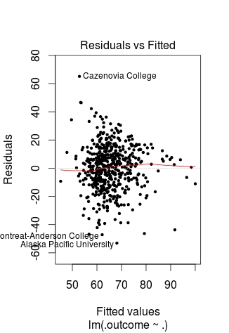
We cannot use a regular plot because are model involves more than two dimensions.  To get around this problem to see are modeling, we will graph fitted values against the residual values. Fitted values are the predict values while residual values are the acutal values from the data. Below is the code followed by the plot.

> CheckModel<-train(Grad.Rate~S.F.Ratio+PhD+Expend, method="lm", data=trainingset)
> DoubleCheckModel<-CheckModel$finalModel
> plot(DoubleCheckModel, 1, pch=19, cex=0.5)
Rplot01

Here is what happened

  1. We created the variable ‘CheckModel’.  In this variable, we used the ‘train’ function to create a linear model with all of our variables
  2. We then created the variable ‘DoubleCheckModel’ which includes the information from ‘CheckModel’ plus the new column of ‘finalModel’
  3. Lastly, we plot ‘DoubleCheckModel’

The regression line was automatically added for us. As you can see, the model does not predict much but shows some linearity.

Predict with Model

We will now do one prediction. We want to know the graduation rate when we have the following information

  • Student-to-faculty ratio = 33
  • Phd percent = 76
  • Expenditures per Student = 11000

Here is the code with the answer

> newdata<-data.frame(S.F.Ratio=33, PhD=76, Expend=11000)
> predict(TrainingModel, newdata)
       1 
57.04367

To put it simply, if the student-to-faculty ratio is 33, the percentage of PhD faculty is 76%, and the expenditures per student is 11,000, we can expect 57% of the students to graduate.

Testing

We will now test our model with the testing dataset. We will calculate the RMSE. Below is the code for creating the testing model followed by the codes for calculating each RMSE.

> TestingModel<-lm(Grad.Rate~S.F.Ratio+PhD+Expend, data=testingset)
> sqrt(sum((TrainingModel$fitted-trainingset$Grad.Rate)^2))
[1] 369.4451
> sqrt(sum((TestingModel$fitted-testingset$Grad.Rate)^2))
[1] 219.4796

Here is what happened

  1. We created the ‘TestingModel’ by using the same model as before but using the ‘testingset’ instead of the ‘trainingset’.
  2. The next two lines of codes should look familiar.
  3. From this output the performance of the model improvement on the testing set since the RMSE is lower than compared to the training results.

Conclusion

This post attempted to explain how to predict and assess models with multiple variables. Although complex for some, prediction is a valuable statistical tool in many situations.

Using Regression for Prediction in R

In the last post about R, we looked at plotting information to make predictions. We will now look at an example of making predictions using regression.

We will use the same data as last time with the help of the ‘caret’ package as well. The code below sets up the seed and the training and testing set we need.

> library(caret); library(ISLR); library(ggplot2)
> data("College");set.seed(1)
> PracticeSet<-createDataPartition(y=College$Grad.Rate,  +                                  p=0.5, list=FALSE) > TrainingSet<-College[PracticeSet, ]; TestingSet<- +         College[-PracticeSet, ] > head(TrainingSet)

The code above should look familiar from the previous post.

Make the Scatterplot

We will now create the scatterplot showing the relationship between “S.F. Ratio” and “Grad.Rate” with the code below and the scatterplot.

> plot(TrainingSet$S.F.Ratio, TrainingSet$Grad.Rate, pch=5, col="green", 
xlab="Student Faculty Ratio", ylab="Graduation Rate")

Rplot10

Here is what we did

  1. We used the ‘plot’ function to make this scatterplot. The x variable was ‘S.F.Ratio’ of the ‘TrainingSet’ the y variable was ‘Grad.Rate’.
  2. We picked the type of dot to use using the ‘pch’ argument and choosing ’19’
  3. Next, we chose a color and labeled each axis

Fitting the Model

We will now develop the linear model. This model will help us to predict future models. Furthermore, we will compare the model of the Training Set with the Test Set. Below is the code for developing the model.

> TrainingModel<-lm(Grad.Rate~S.F.Ratio, data=TrainingSet)
> summary(TrainingModel)

How to interpret this information was presented in a previous post. However, to summarize, we can say that when the student to faculty ratio increases one the graduation rate decreases 1.29. In other words, an increase in the student to faculty ratio leads to decrease in the graduation rate.

Adding the Regression Line to the Plot

Below is the code for adding the regression line followed by the scatterplot

> plot(TrainingSet$S.F.Ratio, TrainingSet$Grad.Rate, pch=19, col="green", xlab="Student Faculty Ratio", ylab="Graduation Rate")
> lines(TrainingSet$S.F.Ratio, TrainingModel$fitted, lwd=3)

Rplot01

Predicting New Values

With our model complete we can now predict values. For our example, we will only predict one value. We want to know what the graduation rate would be if we have a student to faculty ratio of 33. Below is the code for this with the answer

> newdata<-data.frame(S.F.Ratio=33)
> predict(TrainingModel, newdata)
      1 
40.6811

Here is what we did

  1. We made a variable called ‘newdata’ and stored a data frame in it with a variable called ‘S.F.Ratio’ with a value of 33. This is x value
  2. Next, we used the ‘predict’ function from the ‘caret’ package to determine what the graduation rate would be if the student to faculty ratio is 33. To do this we told caret to use the ‘TrainingModel’ we developed using regression and to run this model with the information in the ‘newdata’ dataframe
  3. The answer was 40.68. This means that if the student to faculty ratio is 33 at a university then the graduation rate would be about 41%.

Testing the Model

We will now test the model we made with the training set with the testing set. First, we will make a visual of both models by using the “plot” function. Below is the code follow by the plots.

par(mfrow=c(1,2))
plot(TrainingSet$S.F.Ratio,
TrainingSet$Grad.Rate, pch=19, col=’green’,  xlab=”Student Faculty Ratio”, ylab=’Graduation Rate’)
lines(TrainingSet$S.F.Ratio,  predict(TrainingModel), lwd=3)
plot(TestingSet$S.F.Ratio,  TestingSet$Grad.Rate, pch=19, col=’purple’,
xlab=”Student Faculty Ratio”, ylab=’Graduation Rate’)
lines(TestingSet$S.F.Ratio,  predict(TrainingModel, newdata = TestingSet),lwd=3)

Rplot02.jpeg

In the code, all that is new is the “par” function which allows us to see to plots at the same time. We also used the ‘predict’ function to set the plots. As you can see, the two plots are somewhat differ based on a visual inspection. To determine how much so, we need to calculate the error. This is done through computing the root mean square error as shown below.

> sqrt(sum((TrainingModel$fitted-TrainingSet$Grad.Rate)^2))
[1] 328.9992
> sqrt(sum((predict(TrainingModel, newdata=TestingSet)-TestingSet$Grad.Rate)^2))
[1] 315.0409

The main take away from this complicated calculation is the number 328.9992 and 315.0409. These numbers tell you the amount of error in the training model and testing model. The lower the number the better the model. Since the error number in the testing set is lower than the training set we know that our model actually improves when using the testing set. This means that our model is beneficial in assessing graduation rates. If there were problems we may consider using other variables in the model.

Conclusion

This post shared ways to develop a regression model for the purpose of prediction and for model testing.

Using Plots for Prediction in R

It is common in machine learning to look at the training set of your data visually. This helps you to decide what to do as you begin to build your model.  In this post, we will make several different visual representations of data using datasets available in several R packages.

We are going to explore data in the “College” dataset in the “ISLR” package. If you have not done so already, you need to download the “ISLR” package along with “ggplot2” and the “caret” package.
Once these packages are installed in R you want to look at a summary of the variables use the summary function as shown below.

summary(College)

You should get a printout of information about 18 different variables. Based on this printout, we want to explore the relationship between graduation rate “Grad.Rate” and student to faculty ratio “S.F.Ratio”. This is the objective of this post.

Next, we need to create a training and testing dataset below is the code to do this.

> library(ISLR);library(ggplot2);library(caret)
> data("College")
> PracticeSet<-createDataPartition(y=College$Enroll, p=0.7, +                                  list=FALSE) > trainingSet<-College[PracticeSet,] > testSet<-College[-PracticeSet,] > dim(trainingSet); dim(testSet)
[1] 545  18
[1] 232  18

The explanation behind this code was covered in predicting with caret so we will not explain it again. You just need to know that the dataset you will use for the rest of this post is called “trainingSet”.

Developing a Plot

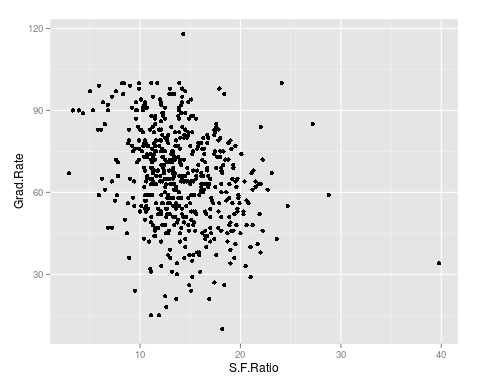
We now want to explore the relationship between graduation rates and student to faculty ratio. We will be used the ‘ggpolt2’  package to do this. Below is the code for this followed by the plot.

qplot(S.F.Ratio, Grad.Rate, data=trainingSet)
Rplot10
As you can see, there appears to be a negative relationship between student faculty ratio and grad rate. In other words, as the ration of student to faculty increases there is a decrease in the graduation rate.

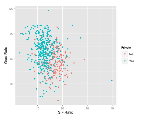
Next, we will color the plots on the graph based on whether they are a public or private university to get a better understanding of the data. Below is the code for this followed by the plot.

> qplot(S.F.Ratio, Grad.Rate, colour = Private, data=trainingSet)
Rplot.jpeg
It appears that private colleges usually have lower student to faculty ratios and also higher graduation rates than public colleges

Add Regression Line

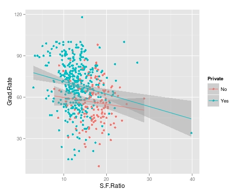
We will now plot the same data but will add a regression line. This will provide us with a visual of the slope. Below is the code followed by the plot.

> collegeplot<-qplot(S.F.Ratio, Grad.Rate, colour = Private, data=trainingSet) > collegeplot+geom_smooth(method = ‘lm’,formula=y~x)
Rplot01.jpeg
Most of this code should be familiar to you. We saved the plot as the variable ‘collegeplot’. In the second line of code, we add specific coding for ‘ggplot2’ to add the regression line. ‘lm’ means linear model and formula is for creating the regression.

Cutting the Data

We will now divide the data based on the student-faculty ratio into three equal size groups to look for additional trends. To do this you need the “Hmisc” packaged. Below is the code followed by the table

> library(Hmisc)
> divide_College<-cut2(trainingSet$S.F.Ratio, g=3)
> table(divide_College)
divide_College
[ 2.9,12.3) [12.3,15.2) [15.2,39.8] 
        185         179         181

Our data is now divided into three equal sizes.

Box Plots

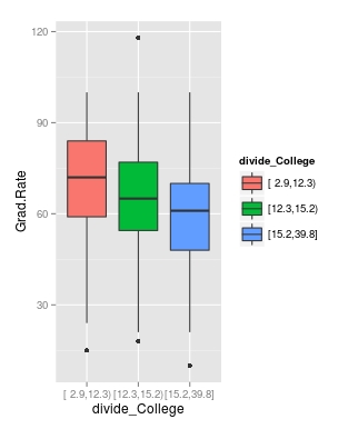
Lastly, we will make a box plot with our three equal size groups based on student-faculty ratio. Below is the code followed by the box plot

CollegeBP<-qplot(divide_College, Grad.Rate, data=trainingSet, fill=divide_College, geom=c(“boxplot”)) > CollegeBP
Rplot02
As you can see, the negative relationship continues even when student-faculty is divided into three equally size groups. However, our information about private and public college is missing. To fix this we need to make a table as shown in the code below.

> CollegeTable<-table(divide_College, trainingSet$Private)
> CollegeTable
              
divide_College  No Yes
   [ 2.9,12.3)  14 171
   [12.3,15.2)  27 152
   [15.2,39.8] 106  75

This table tells you how many public and private colleges there based on the division of the student-faculty ratio into three groups. We can also get proportions by using the following

> prop.table(CollegeTable, 1)
              
divide_College         No        Yes
   [ 2.9,12.3) 0.07567568 0.92432432
   [12.3,15.2) 0.15083799 0.84916201
   [15.2,39.8] 0.58563536 0.41436464

In this post, we found that there is a negative relationship between student-faculty ratio and graduation rate. We also found that private colleges have a lower student-faculty ratio and a higher graduation rate than public colleges. In other words, the status of a university as public or private moderates the relationship between student-faculty ratio and graduation rate.

You can probably tell by now that R can be a lot of fun with some basic knowledge of coding.

Predicting with Caret

In this post, we will explore the use of the caret package for developing algorithms for use in machine learning. The caret package is particularly useful for processing data before the actual analysis of the algorithm.

When developing algorithms is common practice to divide the data into a training a testing subsamples. The training subsample is what is used to develop the algorithm while the testing sample is used to assess the predictive power of the algorithm. There are many different ways to divide a sample into a testing and training set and one of the main benefits of the “caret” package is in dividing the sample.

In the example we will use, we will return to the “kearnlab” example and this develop an algorithm after sub-setting the sample to have a training data set and a testing data set.

First, you need to download the ‘caret’ and ‘kearnlab’ package if you have not done so. After that below is the code for subsetting the ‘spam’ data from the ‘kearnlab’ package.

inTrain<- createDataPartition(y=spam$type, p=0.75, 
list=FALSE)
training<-spam[inTrain,]
testing<-spam[-inTrain,] 
dim(training)

Here is what we did

  1. We created the variable ‘inTrain’
  2. In the variable ‘inTrain’ we told R to make a partition in the data use the ‘createDataPartition’ function. I the parenthesis we told r to look at the dataset ‘spam’ and to examine the variable ‘type’. Then we told are to pull 75% of the data in ‘type’ and copy it to the ‘inTrain’ variable we created. List = False tells R not to make a list. If you look closely, you will see that the variable ‘type’ is being set as the y variable in the ‘inTrain’ data set. This means that all the other variables in the data set will be used as predictors. Also, remember that the ‘type’ variable has two outcomes “spam” or “nonspam”
  3. Next, we created the variable ‘training’ which is the dataset we will use for developing our algorithm. To make this we take the original ‘spam’ data and subset the ‘inTrain’ partition. Now all the data that is in the ‘inTrain’ partition is now in the ‘training’ variable.
  4. Finally, we create the ‘testing’ variable which will be used for testing the algorithm. To make this variable, we tell R to take everything that was not assigned to the ‘inTrain’ variable and put it into the ‘testing’ variable. This is done through the use of a negative sign
  5. The ‘dim’ function just tells us how many rows and columns we have as shown below.
[1] 3451   58

As you can see, we have 3451 rows and 58 columns. Rows are for different observations and columns are for the variables in the data set.

Now to make the model. We are going to bootstrap our sample. Bootstrapping involves random sampling from the sample with replacement in order to assess the stability of the results. Below is the code for the bootstrap and model development followed by an explanation.

set.seed(32343)
SpamModel<-train(type ~., data=training, method="glm")
SpamModel

Here is what we did,

  1. Whenever you bootstrap, it is wise to set the seed. This allows you to reproduce the same results each time. For us, we set the seed to 32343
  2. Next, we developed the actual model. We gave the model the name “SpamModel” we used the ‘train’ function. Inside the parenthesis, we tell r to set “type” as the y variable and then use ~. which is a shorthand for using all other variables in the model as predictor variables. Then we set the data to the ‘training’ data set and indicate that the method is ‘glm’ which means generalized linear model.
  3. The output for the analysis is available at the link SpamModel

There is a lot of information but the most important information for us is the accuracy of the model which is 91.3%. The kappa stat tells us what the expected accuracy of the model is which is 81.7%. This means that our model is a little bit better than the expected accuracy.

For our final trick, we will develop a confusion matrix to assess the accuracy of our model using the ‘testing’ sample we made earlier. Below is the code

SpamPredict<-predict(SpamModel, newdata=testing)
confusionMatrix(SpamPredict, testing$type)

Here is what we did,

  1. We made a variable called ‘SpamPredict’. We use the function ‘predict’ using the ‘SpamModel’ with the new data called ‘testing’.
  2. Next, we make matrix using the ‘confusionMatrix’ function using the new model ‘SpamPredict’ based on the ‘testing’ data on the ‘type’ variable. Below is the output

Reference

  1. Prediction nonspam spam
       nonspam     657   35
       spam         40  418
                                              
                   Accuracy : 0.9348          
                     95% CI : (0.9189, 0.9484)
        No Information Rate : 0.6061          
        P-Value [Acc > NIR] : <2e-16          
                                              
                      Kappa : 0.8637          
     Mcnemar's Test P-Value : 0.6442          
                                              
                Sensitivity : 0.9426          
                Specificity : 0.9227          
             Pos Pred Value : 0.9494          
             Neg Pred Value : 0.9127          
                 Prevalence : 0.6061          
             Detection Rate : 0.5713          
       Detection Prevalence : 0.6017          
          Balanced Accuracy : 0.9327          
                                              
           'Positive' Class : nonspam

    The accuracy of the model actually improved to 93% on the test data. The other values such as sensitivity and specificity have to do with such things as looking at correct classifications divided by false negatives and other technical matters. As you can see, machine learning is a somewhat complex experience

Simple Prediction

Prediction is one of the key concepts of machine learning. Machine learning is a field of study that is focused on the development of algorithms that can be used to make predictions.

Anyone who has shopped online at has experienced machine learning. When you make a purchase at an online store, the website will recommend additional purchases for you to make. Often these recommendations are based on whatever you have purchased or whatever you click on while at the site.

There are two common forms of machine learning, unsupervised and supervised learning. Unsupervised learning involves using data that is not cleaned and labeled and attempts are made to find patterns within the data. Since the data is not labeled, there is no indication of what is right or wrong

Supervised machine learning is using cleaned and properly labeled data. Since the data is labeled there is some form of indication whether the model that is developed is accurate or not. If the is incorrect then you need to make adjustments to it. In other words, the model learns based on its ability to accurately predict results. However, it is up to the human to make adjustments to the model in order to improve the accuracy of it.

In this post, we will look at using R for supervised machine learning. The definition presented so far will make more sense with an example.

The Example

We are going to make a simple prediction about whether emails are spam or not using data from kern lab.

The first thing that you need to do is to install and load the “kernlab” package using the following code

install.packages("kernlab")
library(kernlab)

If you use the “View” function to examine the data you will see that there are several columns. Each column tells you the frequency of a word that kernlab found in a collection of emails. We are going to use the word/variable “money” to predict whether an email is spam or not. First, we need to plot the density of the use of the word “money” when the email was not coded as spam. Below is the code for this.

plot(density(spam$money[spam$type=="nonspam"]),
 col='blue',main="", xlab="Frequency of 'money'")

This is an advance R post so I am assuming you can read the code. The plot should look like the following.

Rplot10

As you can see, money is not used to frequently in emails that are not spam in this dataset. However, you really cannot say this unless you compare the times ‘money’ is labeled nonspam to the times that it is labeled spam. To learn this we need to add a second line that explains to us when the word ‘money’ is used and classified as spam. The code for this is below with the prior code included.

plot(density(spam$money[spam$type=="nonspam"]),
 col='blue',main="", xlab="Frequency of 'money'")
lines(density(spam$money[spam$type=="spam"]), col="red")

Your new plot should look like the following

Rplot10

If you look closely at the plot doing a visual inspection, where there is a separation between the blue line for nonspam and the red line for spam is the cutoff point for whether an email is spam or not. In other words, everything inside the arc is labeled correctly while the information outside the arc is not.

The next code and graph show that this cutoff point is around 0.1. This means that any email that has on average more than 0.1 frequency of the word ‘money’ is spam. Below is the code and the graph with the cutoff point indicated by a black line.

plot(density(spam$money[spam$type=="nonspam"]),
 col='blue',main="", xlab="Frequency of 'money'")
lines(density(spam$money[spam$type=="spam"]), col="red")
abline(v=0.1, col="black", lw= 3)

Rplot10.jpeg Now we need to calculate the accuracy of the use of the word ‘money’ to predict spam. For our current example, we will simply use in “ifelse” function. If the frequency is greater than 0.1.

We then need to make a table to see the results. The code for the “ifelse” function and the table are below followed by the table.

predict<-ifelse(spam$money > 0.1, "spam","nonspam")
table(predict, spam$type)/length(spam$type)
predict       nonspam        spam
  nonspam 0.596392089 0.266898500
  spam    0.009563138 0.127146273

Based on the table that I am assuming you can read, our model accurately calculates that an email is spam about 71% (0.59 + 0.12) of the time based on the frequency of the word ‘money’ being greater than 0.1.

Of course, for this to be true machine learning we would repeat this process by trying to improve the accuracy of the prediction. However, this is an adequate introduction to this topic.

Intro to Making Plots in R

One of the strongest points of R in the opinion of many are the various features for creating graphs and other visualizations of data. In this post, we begin to look at using the various visualization features of R. Specifically, we are going to do the following

  • Using data in R to display graph
  • Add text to a graph
  • Manipulate the appearance of data in a graph

Using Plots

The ‘plot’ function is one of the basic options for graphing data. We are going to go through an example using the ‘islands’ data that comes with the R software. The ‘islands’ software includes lots of data, in particular, it contains data on the lass mass of different islands. We want to plot the land mass of the seven largest islands. Below is the code for doing this.

islandgraph<-head(sort(islands, decreasing=TRUE), 7)
plot(islandgraph, main = "Land Area", ylab = "Square Miles")
text(islandgraph, labels=names(islandgraph), adj=c(0.5,1))

Here is what we did

  1. We made the variable ‘islandgraph’
  2. In the variable ‘islandgraph’ We used the ‘head’ and the ‘sort’ function. The sort function told R to sort the ‘island’ data by decreasing value ( this is why we have the decreasing argument equaling TRUE). After sorting the data, the ‘head’ function tells R to only take the first 7 values of ‘island’ (see the 7 in the code) after they are sorted by decreasing order.
  3. Next, we use the plot function to plot are information in the ‘islandgraph’ variable. We also give the graph a title using the ‘main’ argument followed by the title. Following the title, we label the y-axis using the ‘ylab’ argument and putting in quotes “Square Miles”.
  4. The last step is to add text to the information inside the graph for clarity. Using the ‘text’ function, we tell R to add text to the ‘islandgraph’ variable using the names from the ‘islandgraph’ data which uses the code ‘label=names(islandgraph)’. Remember the ‘islandgraph’ data is the first 7 islands from the ‘islands’ dataset.
  5. After telling R to use the names from the islandgraph dataset we then tell it to place the label a little of center for readability reasons with the code ‘adj = c(0.5,1).

Below is what the graph should look like.

Rplotblog

Changing Point Color and Shape in a Graph

For visual purposes, it may be beneficial to manipulate the color and appearance of several data points in a graph. To do this, we are going to use the ‘faithful’ dataset in R. The ‘faithful’ dataset indicates the length of eruption time and how long people had to wait for the eruption. The first thing we want to do is plot the data using the “plot” function.

Rplot

As you see the data, there are two clear clusters. One contains data from 1.5-3 and the second cluster contains data from 3.5-5. To help people to see this distinction we are going to change the color and shape of the data points in the 1.5-3 range. Below is the code for this.

eruption_time<-with(faithful, faithful[eruptions < 3, ])
plot(faithful)
points(eruption_time, col = "blue", pch = 24)

Here is what we did

  1. We created a variable named ‘eruption_time’
  2. In this variable, we use the ‘with’ function. This allows us to access columns in the dataframe without having to use the $ sign constantly. We are telling R to look at the ‘faithful’ dataframe and only take the information from faithful that has eruptions that are less than 3. All of this is indicated in the first line of code above.
  3. Next, we plot ‘faithful’ again
  4. Last, we add the points from are ‘eruption_time’ variable and we tell R to color these points blue and to use a different point shape by using the ‘pch = 24’ argument
  5. The results are below

last.jpeg

Conclusion

In this post, we learned the following

  • How to make a graph
  • How to add a title and label the y-axis
  • How to change the color and shape of the data points in a graph

Simple Regression in R

In this post, we will look at how to perform a simple regression using R. We will use a built-in dataset in R called ‘mtcars.’ There are several variables in this dataset but we will only use ‘wt’ which stands for the weight of the cars and ‘mpg’ which stands for miles per gallon.

Developing the Model

We want to know the association or relationship between the weight of a car and miles per gallon. We want to see how much of the variance of ‘mpg’ is explained by ‘wt’. Below is the code for this.

> Carmodel <- lm(mpg ~ wt, data = mtcars)

Here is what we did

  1. We created the variable ‘Carmodel’ to store are information
  2. Inside this variable, we used the ‘lm’ function to tell R to make a linear model.
  3. Inside the function, we put ‘mpg ~ wt’ the ‘~’ sign means ’tilda’ in English and is used to indicate that ‘mpg’ is a function of ‘wt’. This section is the actual notation for the regression model.
  4. After the comma, we see ‘data = mtcars’ this is telling R to use the ‘mtcar’ dataset.

Seeing the Results

Once you pressed enter you probably noticed nothing happens. The model ‘Carmodel’ was created but the results have not been displayed. Below is various information you can extract from your model.

The ‘summary’ function is useful for pulling most of the critical information. Below is the code for the output.

> summary(Carmodel)

Call:
lm(formula = mpg ~ wt, data = mtcars)

Residuals:
    Min      1Q  Median      3Q     Max 
-4.5432 -2.3647 -0.1252  1.4096  6.8727 

Coefficients:
            Estimate Std. Error t value Pr(>|t|)    
(Intercept)  37.2851     1.8776  19.858  < 2e-16 ***
wt           -5.3445     0.5591  -9.559 1.29e-10 ***
---
Signif. codes:  0 ‘***’ 0.001 ‘**’ 0.01 ‘*’ 0.05 ‘.’ 0.1 ‘ ’ 1

Residual standard error: 3.046 on 30 degrees of freedom
Multiple R-squared:  0.7528,	Adjusted R-squared:  0.7446 
F-statistic: 91.38 on 1 and 30 DF,  p-value: 1.294e-10

We are not going to explain the details of the output (please see simple regression). The results indicate a model that explains 75% of the variance or has an r-square of 0.75. The model is statistically significant and the equation of the model is -5.45x + 37.28 = y

Plotting the Model

We can also plot the model using the code below

> coef_Carmodel<-coef(Carmodel)
> plot(mpg ~ wt, data = mtcars)
> abline(a = coef_Carmodel[1], b = coef_Carmodel[2])

Here is what we did

  1. We made the variable ‘coef_Carmodel’ and stored the coefficients (intercept and slope) of the ‘Carmodel’ using the ‘coef’ function. We will need this information soon.
  2. Next, we plot the ‘mtcars’ dataset using ‘mpg’ and ‘wt’.
  3. To add the regression line we use the ‘abline’ function. To add the intercept and slope we use a = the intercept from our ‘coef_Carmodel’ variable which is subset [1] from this variable. For slope, we follow the same process but use a [2]. This will add the line and your graph should look like the following.

Rplot10

From the visual, you can see that as weight increases there is a decrease in miles per gallon.

Conclusion

R is capable of much more complex models than the simple regression used here. However, understanding the coding for simple modeling can help in preparing you for much more complex forms of statistical modeling.

ANOVA with R

Analysis of variance (ANOVA) is used when you want to see if there is a difference in the means of three or more groups due to some form of treatment(s). In this post, we will look at conducting an ANOVA calculation using R.

We are going to use a dataset that is already built into R called ‘InsectSprays.’ This dataset contains information on different insecticides and their ability to kill insects. What we want to know is which insecticide was the best at killing insects.

In the dataset ‘InsectSprays’, there are two variables, ‘count’, which is the number of dead bugs, and ‘spray’ which is the spray that was used to kill the bug. For the ‘spray’ variable there are six types label A-F. There are 72 total observations for the six types of spray which comes to about 12 observations per spray.

Building the Model

The code for calculating the ANOVA is below

> BugModel<- aov(count ~ spray, data=InsectSprays)
> BugModel
Call:
   aov(formula = count ~ spray, data = InsectSprays)

Terms:
                   spray Residuals
Sum of Squares  2668.833  1015.167
Deg. of Freedom        5        66

Residual standard error: 3.921902
Estimated effects may be unbalanced

Here is what we did

  1. We created the variable ‘BugModel’
  2. In this variable, we used the function ‘aov’ which is the ANOVA function.
  3. Within the ‘aov’ function we told are to determine the count by the difference sprays that is what the ‘~’ tilde operator does.
  4. After the comma, we told R what dataset to use which was “InsectSprays.”
  5. Next, we pressed ‘enter’ and nothing happens. This is because we have to make R print the results by typing the name of the variable “BugModel” and pressing ‘enter’.
  6. The results do not tell us anything too useful yet. However, now that we have the ‘BugModel’ saved we can use this information to find the what we want.

Now we need to see if there are any significant results. To do this we will use the ‘summary’ function as shown in the script below

> summary(BugModel)
            Df Sum Sq Mean Sq F value Pr(>F)    
spray        5   2669   533.8    34.7 <2e-16 ***
Residuals   66   1015    15.4                   
---
Signif. codes:  0 ‘***’ 0.001 ‘**’ 0.01 ‘*’ 0.05 ‘.’ 0.1 ‘ ’ 1

These results indicate that there are significant results in the model as shown by the p-value being essentially zero (Pr(>F)). In other words, there is at least one mean that is different from the other means statistically.

We need to see what the means are overall for all sprays and for each spray individually. This is done with the following script

> model.tables(BugModel, type = 'means')
Tables of means
Grand mean
    
9.5 

 spray 
spray
     A      B      C      D      E      F 
14.500 15.333  2.083  4.917  3.500 16.667

The ‘model.tables’ function tells us the means overall and for each spray. As you can see, it appears spray F is the most efficient at killing bugs with a mean of 16.667.

However, this table does not indicate the statistically significance. For this we need to conduct a post-hoc Tukey test. This test will determine which mean is significantly different from the others. Below is the script

> BugSpraydiff<- TukeyHSD(BugModel)
> BugSpraydiff
  Tukey multiple comparisons of means
    95% family-wise confidence level

Fit: aov(formula = count ~ spray, data = InsectSprays)

$spray
           diff        lwr       upr     p adj
B-A   0.8333333  -3.866075  5.532742 0.9951810
C-A -12.4166667 -17.116075 -7.717258 0.0000000
D-A  -9.5833333 -14.282742 -4.883925 0.0000014
E-A -11.0000000 -15.699409 -6.300591 0.0000000
F-A   2.1666667  -2.532742  6.866075 0.7542147
C-B -13.2500000 -17.949409 -8.550591 0.0000000
D-B -10.4166667 -15.116075 -5.717258 0.0000002
E-B -11.8333333 -16.532742 -7.133925 0.0000000
F-B   1.3333333  -3.366075  6.032742 0.9603075
D-C   2.8333333  -1.866075  7.532742 0.4920707
E-C   1.4166667  -3.282742  6.116075 0.9488669
F-C  14.5833333   9.883925 19.282742 0.0000000
E-D  -1.4166667  -6.116075  3.282742 0.9488669
F-D  11.7500000   7.050591 16.449409 0.0000000
F-E  13.1666667   8.467258 17.866075 0.0000000

There is a lot of information here. To make things easy, wherever there is a p adj of less than 0.05 that means that there is a difference between those two means. For example, bug spray F and E have a difference of 13.16 that has a p adj of zero. So these two means are really different statistically.This chart also includes the lower and upper bounds of the confidence interval.

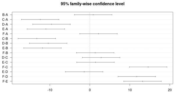
The results can also be plotted with the script below

> plot(BugSpraydiff, las=1)

Below is the plot

Rplot10

Conclusion

ANOVA is used to calculate if there is a difference of means among three or more groups. This analysis can be conducted in R using various scripts and codes.

Calculating Chi-Square in R

There are times when conducting research that you want to know if there is a difference in categorical data. For example, is there a difference in the number of men who have blue eyes and who have brown eyes. Or is there a relationship between gender and hair color. In other words, is there a difference in the count of a particular characteristic or is there a relationship between two or more categorical variables.

In statistics, the chi-square test is used to compare categorical data. In this post, we will look at how you can use the chi-square test in R.

For our example, we are going to use data that is already available in R called “HairEyeColor”. Below is the data

> HairEyeColor
, , Sex = Male

       Eye
Hair    Brown Blue Hazel Green
  Black    32   11    10     3
  Brown    53   50    25    15
  Red      10   10     7     7
  Blond     3   30     5     8

, , Sex = Female

       Eye
Hair    Brown Blue Hazel Green
  Black    36    9     5     2
  Brown    66   34    29    14
  Red      16    7     7     7
  Blond     4   64     5     8

As you can see, the data comes in the form of a list and shows hair and eye color for men and women in separate tables. The current data is unusable for us in terms of calculating differences. However, by using the ‘marign.table’ function we can make the data useable as shown in the example below.

> HairEyeNew<- margin.table(HairEyeColor, margin = c(1,2))
> HairEyeNew
       Eye
Hair    Brown Blue Hazel Green
  Black    68   20    15     5
  Brown   119   84    54    29
  Red      26   17    14    14
  Blond     7   94    10    16

Here is what we did. We created the variable ‘HairEyeNew’ and we stored the information from ‘HairEyeColor’ into one table using the ‘margin.table’ function. The margin was set 1,2 for the table.

Now all are data from the list are combined into one table.

We now want to see if there is a particular relationship between hair and eye color that is more common. To do this, we calculate the chi-square statistic as in the example below.

> chisq.test(HairEyeNew)

	Pearson's Chi-squared test

data:  HairEyeNew
X-squared = 138.29, df = 9, p-value < 2.2e-16

The test tells us that one or more of the relationships are more common than others within the table. To determine which relationship between hair and eye color is more common than the rest we will calculate the proportions for the table as seen below.

> HairEyeNew/sum(HairEyeNew)
       Eye
Hair          Brown        Blue       Hazel       Green
  Black 0.114864865 0.033783784 0.025337838 0.008445946
  Brown 0.201013514 0.141891892 0.091216216 0.048986486
  Red   0.043918919 0.028716216 0.023648649 0.023648649
  Blond 0.011824324 0.158783784 0.016891892 0.027027027

As you can see from the table, brown hair and brown eyes are the most common (0.20 or 20%) flowed by blond hair and blue eyes (0.15 or 15%).

Conclusion

The chi-square serves to determine differences among categorical data. This tool is useful for calculating the potential relationships among non-continuous variables

Comparing Samples in R

Comparing groups is a common goal in statistics. This is done to see if there is a difference between two groups. Understanding the difference can lead to insights based on statistical results. In this post, we will examine the following statistical test for comparing samples.

  • t-test/Wilcoxon test
  • Paired t-test

T-test & Wilcoxon Test

The T-test indicates if there is a significant statistical difference between two groups. This is useful if you know what the difference between the two groups are. For example, if you are measuring height of men and women, if you find that men are taller through a t-test, you can state that gender influences height because the only difference between men and women in this example is their gender.

Below is an example of conducting a t-test in R. In the example, we are looking at if there is a difference in body temperature between beavers who are active versus beavers who are not.

> t.test(temp ~ activ, data = beaver2)

	Welch Two Sample t-test

data:  temp by activ
t = -18.548, df = 80.852, p-value < 2.2e-16
alternative hypothesis: true difference in means is not equal to 0
95 percent confidence interval:
 -0.8927106 -0.7197342
sample estimates:
mean in group 0 mean in group 1 
       37.09684        37.90306

Here is what happened

  1. We use the ‘t.test’ function
  2. Within the ‘t.test’ function we indicate that we want to if there is a difference in ‘temp’ when compared on the factor variable ‘activ’ in the data ‘beaver2’
  3. The output provides a lot of information. The t-stat is -18.58 any number at + 1.96 indicates statistical difference.
  4. Df stands for degrees of freeedom and is used to determine the t-stat and p-value.
  5. The p-value is basically zero. Anything less than 0.05 is considered statistically significant.
  6. Next, we have the 95% confidence interval, which is the range of the difference of the means of the two groups in the population.
  7. Lastly, we have the means of each group. Group 0, the inactive group. had a mean of 37.09684. Group 1. the active group, has a mean of  37.90306.

T-test assumes that the data is normally distributed. When normality is a problem, it is possible to use the Wilcoxon test instead. Below is the script for the Wilcoxon Test using the same example.

> wilcox.test(temp ~ activ, data = beaver2)

	Wilcoxon rank sum test with continuity correction

data:  temp by activ
W = 15, p-value < 2.2e-16
alternative hypothesis: true location shift is not equal to 0

A closer look at the output indicates the same results for the most part. Instead of the t-stat the W-stat is used but the p value is the same for both test.

Paired T-Test

A paired t-test is used when you want to compare how the same group of people respond to different interventions. For example, you might use this for a before and after experiment. We will use the ‘sleep’ data in R  to compare a group of people when they receive different types of sleep medication. The script is below

> t.test(extra ~ group, data = sleep, paired = TRUE)

	Paired t-test

data:  extra by group
t = -4.0621, df = 9, p-value = 0.002833
alternative hypothesis: true difference in means is not equal to 0
95 percent confidence interval:
 -2.4598858 -0.7001142
sample estimates:
mean of the differences 
                  -1.58

Here is what happened

  1. We used the ‘t.test’ function and indicate we want to see if ‘extra’ (amount of sleep) is influenced by ‘group’ (two types of sleep medication.
  2. We add the new argument of ‘paired = TRUE’ this tells R that this is a paired test.
  3. The output is the same information as in the regular t.test. The only differences is at the bottom where R only tells you the difference between the two groups and not the means of each. For this example, the people slept about 1 hour and 30 minutes longer on the second sleep medication when compared to the first.

Conclusion

Comparing samples in R is a simple process of understanding what you want to do. With this knowledge, the script and output are not too challenge even for many beginners

Examining Distributions In R

Normal distribution is an important term in statistics. When we say normal distribution, we are speaking of the traditional bell curve concept. Normal distribution is important because it is often an assumption of inferential statistics that the distribution of data points is normal. Therefore, one of the first things you do when analyzing data is to check for normality.

In this post, we will look at the following ways to assess normality.

  • By graph
  • By plots
  • By test

Checking Normality by Graph

The easiest and crudest way to check for normality is visually through the use of histograms. You simply look at the histogram and determine how closely it resembles a bell.

To illustrate this we will use the ‘beaver2’ data that is already loaded into R. This dataset contains five variables “day”, “time”, “temp”, and “activ” for data about beavers. Day indicates what day it was, time indicates what time it was, temp is the temperature of the beavers, and activ is whether the beavers were active when their temperature was taking. We are going to examine the normality of the temperature of active and inactive. Below is the code

> library(lattice)
> histogram(~temp | factor(activ), data = beaver2)
  1. We loaded the ‘lattice’ package. (If you don’t have this package please download)>
  2. We used the histogram function and indicate the variable ‘temp’ then the union ( | ) followed by the factor variable ‘activ’ (0 = inactive, 1 = active)
  3. Next, we indicate the dataset we are using ‘beaver2’
  4. After pressing ‘enter’ you should see the following

Rplot10

As you look at the histograms, you can say that they are somewhat normal. The peaks of the data are a little high in both. Group 1 is more normal than Group 0. The problem with visual inspection is lack of accuracy in interpretation. This is partially solved by using QQ plots.

Checking Normality by Plots

QQplots are useful for comparing your data with a normally distributed theoretical dataset. The QQplot includes a line of a normal distribution and the data points for your data for comparison. The more closely your data follows the line the more normal it is. Below is the code for doing this with our beaver information.

> qqnorm(beaver2$temp[beaver2$activ==1], main = 'Active')
> qqline(beaver2$temp[beaver2$activ==1])

Here is what we did

  1. We used the ‘qqnorm’ function to make the plot
  2. Within the ‘qqnorm’ function we tell are to use ‘temp’ from the ‘beaver2’ dataset.
  3. From the ‘temp’ variable we subset the values that have a 1 in the ‘activ’ variable.
  4. We give the plot a title by adding ‘main = Active’
  5. Finally, we add the ‘qqline’ using most of the previous information.
  6. Below is how the plot should look

R

Going by sight again. The data still looks pretty good. However, one last test will determine conclusively if the dataset is normal or not.

Checking Normality by Test

The Shapiro-Wilks normality test determines the probability that the data is normally distributed. The lower the probability the less likely that the data is normally distributed. Below is the code and results for the Shapiro test.

> shapiro.test(beaver2$temp[beaver2$activ==1])

	Shapiro-Wilk normality test

data:  beaver2$temp[beaver2$activ == 1]
W = 0.98326, p-value = 0.5583

Here is what happened

  1. We use the ‘shapiro.test’ function for ‘temp’ of only the beavers who are active (activ = 1)
  2. R tells us the p-value is 0.55 or 55%
  3. This means that the probability of our data being normally distributed is 55% which means it is highly likely to be normal.

Conclusion

It is necessary to always test the normality of data before data analysis. The tips presented here provide some framework for accomplishing this.

Two-Way Tables in R

A two-way table is used to explain two or more categorical variables at the same time. The difference between a two-way table and a frequency table is that a two-table tells you the number of subjects that share two or more variables in common while a frequency table tells you the number of subjects that share one variable.

For example, a frequency table would be gender. In such a table, you only know how many subjects are male or female. The only variable involved is gender. In a frequency table, you would learn some of the following

  • Total number of men
  • Total number of women
  • Total number of subjects in the study

In a two-way table, you might look at gender and marital status. In such a table you would be able to learn several things

  • Total number of men are married
  • Total number of men are single
  • Total number of women are married
  • Total number of women are single
  • Total number of men
  • Total number of women
  • Total number of married subjects
  • Total number of single subjects
  • Total number of subjects in the study

As such, there is a lot of information in a two-way table. In this post, we will look at the following

  • How to create a table
  • How to add margins to a table
  • How to calculate proportions in a table

Creating a Table

In the example, we are going to look at two categorical variables. One variable is gender and the other is marital status. For gender, the choices are “Male” and Female”. For marital status, the choicest are ‘Married” and “Single”. Below is the code for developing the table.

Marriage_Study<-matrix(c(34,20,19,42), ncol = 2)
colnames(Marriage_Study) <- c('Male', 'Female')
rownames(Marriage_Study) <- c('Married', 'Single')
Marriage_table <- as.table(Marriage_Study)
print(Marriage_table)

There has already been a discussion on creating matrices in R. Therefore, the details of this script will not be explained here.

If you type this correctly and run the script you should see the following

        Male Female
Married   34     19
Single    20     42

This table tells you about married and single people broken down by their gender. For example, 34 males are married.

Adding Margins and Calculating Proportions

A useful addition to a table is to add the margins. The margins tell you the total number of subjects in each row and column of a table. To do this in R use the ‘addmargins’ function as indicated below.

> addmargins(Marriage_table)
        Male Female Sum
Married   34     19  53
Single    20     42  62
Sum       54     61 115

We now know the total number of Married people, Singles, Males, and Females. In addition to the information we already knew.

One more useful piece of information is to calculate the proportions. This will allow us to know what percentage of each two-way possibility makes up the table. To do this we will use the “prop.table” function. Below is the script

> prop.table(Marriage_table)
             Male    Female
Married 0.2956522 0.1652174
Single  0.1739130 0.3652174

As you can see, we now know the proportions of each category in the table.

Conclusions

This post provided information on how to construct and manipulate data that is in a two-way table. Two-way tables are a useful way of describing categorical variables.

Plotting Correlations in R

A correlation indicates the strength of the relationship between two or more variables.  Plotting correlations allows you to see if there is a potential relationship between two variables. In this post, we will look at how to plot correlations with multiple variables.

In R, there is a built-in dataset called ‘iris’. This dataset includes information about different types of flowers. Specifically, the ‘iris’ dataset contains the following variables

  • Sepal.Length
  • Sepal.Width
  • Petal.Length
  • Petal.Width
  • Species

You can confirm this by inputting the following script

> names(iris)
[1] "Sepal.Length" "Sepal.Width"  "Petal.Length" "Petal.Width"  "Species"

We now want to examine the relationship that each of these variables has with each other. In other words, we want to see the relationship of

  • Sepal.Length and Sepal.Width
  • Sepal.Length and Petal.Length
  • Sepal.Length and Petal.Width
  • Sepal.Width and Petal.Length
  • Sepal.Width and Petal.Width
  • Petal.Length and Petal.Width

The ‘Species’ variable will not be a part of our analysis since it is a categorical variable and not a continuous one. The type of correlation we are analyzing is for continuous variables.

We are now going to plot all of these variables above at the same time by using the ‘plot’ function. We also need to tell R not to include the “Species” variable. This is done by adding a subset code to the script. Below is the code to complete this task.

> plot(iris[-5])

Here is what we did

  1. We use the ‘plot’ function and told R to use the “iris” dataset
  2. In brackets, we told R to remove ( – ) the 5th variable, which was species
  3. After pressing enter you should have seen the following

Rplot10

The variable names are placed diagonally from left to right. The x-axis of a plot is determined by variable name in that column. For example,

  • The variable of the x-axis of the first column is ‘Sepal.Length”
  • The variable of the x-axis of the second column is ‘Sepal.Width”
  • The variable of the x-axis of the third column is ‘Petal.Length”
  • The variable of the x-axis of the fourth column is ‘Petal.Width”

The y-axis is determined by the variable that is in the same row as the plot. For example,

  • The variable of the y-axis of the first column is ‘Sepal.Length”
  • The variable of the y-axis of the second column is ‘Sepal.Width”
  • The variable of the y-axis of the third column is ‘Petal.Length”
  • The variable of the y-axis of the fourth column is ‘Petal.Width”

AS you can see, this is the same information. We will now look at a few examples of plots

  • The plot in the first column second row plots “Sepal.Length” as the x-axis and “Sepal.Width” as the y-axis
  • The plot in the first column third row plots “Sepal.Length” as the x-axis and “Petal.Length” as the y-axis
  • The plot in the first column fourth row plots “Sepal.Length” as the x-axis and “Petal.Width” as the y-axis

Hopefully, you can see the pattern. The plots above the diagonal are mirrors of the ones below. If you are familiar with correlational matrices this should not be surprising.

After a visual inspection, you can calculate the actual statistical value of the correlations. To do so use the script below and you will see the table below after it.

> cor(iris[-5])
             Sepal.Length Sepal.Width Petal.Length Petal.Width
Sepal.Length    1.0000000  -0.1175698    0.8717538   0.8179411
Sepal.Width    -0.1175698   1.0000000   -0.4284401  -0.3661259
Petal.Length    0.8717538  -0.4284401    1.0000000   0.9628654
Petal.Width     0.8179411  -0.3661259    0.9628654   1.0000000

As you can see, there are many strong relationships between the variables. For example “Petal.Width” and “Petal.Length” has a correlation of .96, which is almost perfect. This means that when “Petal.Width” grows by one unit “Petal.Length” grows by .96 units.

Conclusion

Plots help you to see the relationship between two variables. After visual inspection, it is beneficial to calculate the actual correlation.

Basics of Histograms and Plots in R

R has many fascinating features for creating histograms and plots. In this post, we will only cover some of the most basic concepts of make histograms and plots in R. The code for the data we are using is available in a previous post.

Making a Histogram

We are going to make a histogram of the ‘mpg’ variable in our ‘cars’ dataset. Below is the code for doing this followed by the actual histogram.

Histogram of mpg variable

Histogram of mpg variable

Here is what we did

  1. We used the ‘hist’ function to create the histogram
  2. Within the hist function we told r to make a histogram of ‘mpg’ variable found in the ‘cars’ dataset.
  3. An additional argument that we added was ‘col’. This argument is used to determine the color of the bars in the histogram. For our example, the color was set to gray.

Plotting Multiple Variables

Before we look at plotting multiple variables you need to make an adjustment to the ‘cyl’ variable in our cars variable. THis variable needs t be changed from a numeric to a factor variable as shown below

cars$cyl<- as.factor(cars$cyl)

Boxplots are an excellent way of comparing groups visually. In this example, we will compare the ‘mpg’ or miles per gallon variable by the ‘cyl’ or number of cylinders in the engine variable in the ‘cars’ dataset. Below is the code and diagram followed by an explanation.

boxplot(mpg ~ cyl, data = cars)

Rplot

Here is what happened.

  1. We use the ‘boxplot’ function
  2. Within this function we tell are to plot mpg and cyl using the tilda  ” ~ ” to tell R to compare ‘mpg’ by the number of cylinders

The box of the boxplot tells you several things

  1. The bottom of the box tells you the 25th percentile
  2. The line in the middle of the box tells you the median
  3. The top of the box tells you the 75th percentile
  4. The bottom line tells you the minimum or lowest value excluding outliers
  5. The top line tells you the maximum or highest value excluding outliers

In order boxplot above, there are three types of cylinders 4, 6, and 8. For 4 cylinders the 25th percentile is about 23 mpg, the 50th percentile is about 26 mpg, while the 75th percentile is about 31 mpg. The minimum value was about 22 and the maximum value was about 35 mpg. A close look at the different blots indicates that four cylinder cars have the best mpg followed by six and finally eight cylinders.

Conclusions

Histograms and boxplots serve the purpose of describing numerical data in a visual manner. Nothing like a picture helps to explain abstract concepts such mean and median.

Describing Categorical Data in R

This post will explain how to create tables, calculate proportions, find the mode, and make plots for categorical variables in R. Before providing examples below is the script needed to setup the data that we are using

cars <- mtcars[c(1,2,9,10)]
cars$am <- factor(cars$am, labels=c('auto', 'manual'))
cars$gear <- ordered(cars$gear)

Tables

Frequency tables are useful for summarizing data that has a limited number of values. It represents how often a particular value appears in a dataset. For example, in our cars dataset, we may want to know how many different kinds of transmission we have. To determine this, use the code below.

> transmission_table <- table(cars$am)
> transmission_table

  auto manual 
    19     13

Here is what we did.

  1. We created the variable ‘transmission_table’
  2. In this variable, we used the ‘table’ function which took information from the ‘am’ variable from the ‘cars’ dataset.
  3. Final we displayed the information by typing ‘transmission_table’ and pressing enter

Proportion

Proportions can also be calculated. A proportion will tell you what percentage of the data belongs to a particular category. Below are the proportions of automatic and manual transmissions in the ‘cats’ dataset.

> transmission_table/sum(transmission_table)

   auto  manual 
0.59375 0.40625

The table above indicates that about 59% of the sample consists of automatic transmissions while about 40% are manual transmissions

Mode

When dealing with categorical variables there is not mean or median. However, it is still possible to calculate the mode, which is the most common value found. Below is the code.

> mode_transmission <-transmission_table ==max(transmission_table)
> names(transmission_table) [mode_transmission]
[1] "auto"

Here is what we did.

  1. We created the variable ‘mode_transmission’ and use the ‘max’ function to calculate the max number of counts in the transmission_table.
  2. Next we calculated the names found in the ‘transmission_table’ but we subsetted the ‘modes_transmission variable
  3. The most common value was ‘auto’ or automatic tradition,

Plots

Plots are one of the funniest capabilities in R. For now, we will only show you how to plot the data that we have been using. What is seen here is only the simplest and basic use of plots in R and there is a much more to it than this. Below is the code for plotting the number of transmission by type in R.

> plot(cars$am)

If you did this correctly you should see the following.

Rplot09

All we did was have R create a visual of the number of auto and manual transmissions.Naturally, you can make plots with continuous variables as well.

Conclusion

This post provided some basic information on various task can be accomplished in R for assessing categorical data. These skills will help researchers to take a sea of data and find simple ways to summarize all of the information.

Describing Continuous Variables in R

In the last post on R, we began to look at how to pull information from a data set. In this post, we will continue this by examining how to describe continuous variables. One of the first steps in any data analysis is to look at the descriptive statistics to determine if there are any problems, errors or issues with normality. Below is the code for the data frame we created.

> cars <- mtcars[c(1,2,9,10)]
> cars$am <- factor(cars$am, labels=c('auto', 'manual'))
> cars$gear <- ordered(cars$gear)

Finding the Mean, Median, Standard Deviation, Range, and Quartiles

The mean is useful to know as it gives you an idea of the centrality of the data. Finding the mean is simple and involves the use of the “mean” function. Keep in mind that there are four variables in our data frame which are mpg, cyl, am, and gear. Only ‘mpg’ has a mean because the other variables are all categorical (cyl, am, and gear). Below is the script for finding the mean of ‘mpg’ with the answer.

> mean(cars$mpg)
[1] 20.09062

The median is the number found exactly in the middle of a dataset. Below is the median of ‘mpg.’

> median(cars$mpg)
[1] 19.2

The answer above indicates that the median of ‘mpg’ is 19.2. This means half the values are above this number while half the values are below it.

Standard deviation is the average amount that a particular data point is different from the mean. For example, if the standard deviation is 3 and the mean is 10 this means that any given data point is either is between 7 and 13 or -3 to  +3 different from the mean. In other words, the standard deviation calculates the average amount of deviance from the mean. Below is a calculation of the standard deviation of the ‘mpg’ in the ‘cars’ data frame using ‘sd’ function.

> sd(cars$mpg)
[1] 6.026948

What this tells is that the average amount of deviance from the mean of 20.09 for ‘mpg’ in the ‘car’ data frame is 6.02. In simple terms, most of the data points are between 14.0 and 26.0 mpg.

Range is the highest and lowest number in a data set. It gives you an idea of the scope of a dataset. This can be calculated in R using the ‘range’ function. Below is the range for ‘mpg’ in the ‘cars’ data frame.

> range(cars$mpg)
[1] 10.4 33.9

These results mean that the lowest ‘mpg’ in the cars data frame is 10.4 while the highest is 33.9. There are no values lower or higher than these.

Lastly, quartiles tell breaks the data into several groups based on a percentage. For example, the 25th percentile gives you a number that tells that 75% of the numbers are higher than it and that 25% is lower. If there are 100 data points in a dataset and the number 25 is the 25th percentile, this means that 75% or 75 numbers are of greater value than 25 and that there are about 25 numbers lower than 25. Below is an example using the ‘mpg’ information from the ‘cars’ data frame using the ‘quantile’ function.

> quantile(cars$mpg)
    0%    25%    50%    75%   100% 
10.400 15.425 19.200 22.800 33.900

In this example above, 15.4 is the 25th percentile. This means that 75% of the values are above 15.4 while 25% are below it. In addition, you may have noticed that the 0% and the 100% are the same as the range. Furthermore, the 50% is the same as the median. In other words, calculating the quartiles gives you the range and median. Therefore, calculating the quartiles saves you time.

Conclusion

These are the basics of describing continuous variables. The next post on R will look at describing categorical variables.

Working with Data in R

In this post and future posts, we will work with actual data that is available in R to apply various skills. For now, we will work with the ‘mtcars’ data that is available in R. This dataset contains information about 32 different cars that were built in the 1970’s.

Often in research, the person who collects the data and the person who analyzes the data (the statistician) are different. This often leads to the statistician getting a lot of missing data that cannot be analyzed in its current state. This leads to the statistician having to clean the data in order to analyze it.

Initial Decisions

One of the first things a statistician does after he has received some data is to see how many different variables there are and perhaps decide if any can be converted to factors. In order to achieve these two goals we need to answer the following questions

  1. How many variables are there? Many functions can answer this question
  2. How many unique values does each variable have? This will tell us if the variable is a candidate for becoming a factor.

Below is the code for doing this with the ‘mtcar’ dataset.

> sapply(mtcars, function(x) length(unique(x)))
 mpg  cyl disp   hp drat   wt qsec   vs   am gear carb 
  25    3   27   22   22   29   30    2    2    3    6

Here is what we did

  1. We used the ‘sapply’ function because we want to apply our function on the whole dataframe at once.
  2. Inside the ‘sapply’ function we tell R that the dataset is ‘mtcars’
  3. Next is the function we want to use. We tell R to use the function ‘x’ which is an anonymous function.
  4. After indicating that the function is anonymous we tell R what is inside the anonymous function.
  5. The anonymous function contains the length function with the unique function within it.
  6. This means that we want the length (or number) of unique values in each variable.

We have the answers to our question

  1. There are eleven variables in the ‘mtcars’ dataset as listed in the table above
  2. The unique values are also listed in the table above.

A common rule of thumb for determining whether to convert a variable to a factor is that the variable has less then 10 unique values. Based on this rule, the cyl, vs, am, gear, and carb variables could be converted to factors. Converting to a factor makes a continuous variable a categorical one and opens up various analysis possibilities.

Preparing Data

Now that we have an idea of what are the characteristics of the dataset we have to decide the following…

  1. What variables are we going to use
  2. What type of analysis are we going to do with the variables we use.

For question 1 we are going to use the 1st (mpg), the 2nd (cyl), the 9th (am) and the 10th (gear) variables for our analysis. Then we are going to make the ‘am’ variable a factor. Lastly, we are going to put in order the values in the ‘gear’ variable. Below is the code

> cars <- mtcars[c(1,2,9,10)]
> cars$am <- factor(cars$am, labels=c('auto', 'manual'))
> cars$gear <- ordered(cars$gear)

Here is what we did

  1. We created the variable ‘cars’ and assigned a subset of variables from the ‘mtcars’ dataset. In particular, we took the  1st (mpg), the 2nd (cyl), the 9th (am) and the 10th (gear) variables from ‘mtcars’ and saved them in ‘cars’
  2. For the ‘am’ variable we converted it to a factor. Data points that were once 0 became ‘auto’ and data points that were once 1 became ‘manual’
  3. We made the ‘gear’ variable an ordered factor this means that 5 is more than 4, 4 is more than 3, etc.

Our next post on R will focus on analyzing the ‘cars’ variable that we created.

Apply Functions in R

The last R post focused on the use of the “for” loop. This option is powerful in repeating an action that cannot be calculated in a vector. However, there are some drawbacks to ‘for’loops that are highly technical and hard to explain to beginners. The problems have something to do with strange results in the workspace and environment.

To deal with the complex problems with ‘for’ loops have the alternative approach of using functions from the apply family. The functions in the apply family provide the same results as a ‘for’ loop without the occasional problem. There are three functions in the apply family and they are

  • apply
  • sapply
  • lapply

We discuss each with a realistic example.

Apply

The ‘apply’ function is useful for producing results for a matrix, array, or data frame. They do this by producing results from the rows and or columns. The results of an ‘apply’ function are always shared as a vector, matrix, or list. Below is an example of the use of an ‘apply’ function.

You make a matrix that contains how many points James, Kevin, Williams have scored in the past three games. Below is the code for this.

> points.per.game<- matrix(c(25,23,32,20,18,24,12,15,16), ncol=3)
> colnames(points.per.game)<-c('James', 'Kevin', 'Williams')
> rownames(points.per.game)<-c('Game1', 'Game2', 'Game3')
> points.per.game
      James Kevin Williams
Game1    25    20       12
Game2    23    18       15
Game3    32    24       16

You want to know the most points James, Kevin, and Williams scored for any game. To do this, you use the ‘apply’ function as follows.

> apply(points.per.game, 2, max)
   James    Kevin Williams 
      32       24       16

Here is what we did

  1. We used the ‘apply’ function and in the parentheses we  put the arguments “points.per.game” as this is the name of the matrix, ‘2’ which tells R to examine the matrix by column, and lastly we used the argument ‘max’ which tells are to find the maximum value in each column.
  2. R prints out the results telling us the most points each player scored regardless of the game.

Sapply

The ‘apply’ function works for multidimensional objects such as matrices, arrays, and data frames. ‘Sapply’ is used for vectors, data frames, and list. ‘Sapply’ is more flexible in that it can be used for single dimension (vectors) and multidimensional (data frames) objects.  The output from using the ‘sapply’ function is always a vector, matrix, or list. Below is an example

Let’s say you make the following data frame

> GameInfo
  points      GameType
1    101          Home
2    115          Away
3     98 International
4     89          Away
5    104          Home

You now want to know what kind of variables you have in the ‘GameInfo’ data frame. You can calculate this one at a time or you can use the following script with the ‘sapply’ function

> sapply(GameInfo, class)
   points  GameType 
"numeric"  "factor"

Here is what we did

  1. We use the ‘sappy’ function and included two arguments. The first is the name of the data frame “GameInfo” the second is the argument ‘class’ which tells R to determine what kind of variable is in the “GameInfo” data frame
  2. The answer is then printed. The variable ‘points’ is a numeric variable while the variable ‘GameType’ is a factor.

lapply

The ‘lapply’ function works exactly like the ‘sapply’ function but always returns a list. See the example below

> lapply(GameInfo, class)
$points
[1] "numeric"

$GameType
[1] "character"

This the same information from the ‘sapply’ example we ran earlier.

Conclusion

The ‘apply’ family serves the purpose of running a loop without the concerns of the ‘for’ loop. This feature is useful for various objects.

Using ‘for’ Loops in R

In our last post on R, we looked at using the ‘switch’ function. The problem with the ‘switch’ function is that you have to input every data point manually. For example, if you have five different values you want to calculate in a function you need to input each value manually until you have calculated all five.

There is a way around this and it involves the use of a ‘for’ loop. A ‘for’ loop is used to repeat an action in R in a vector. This allows you to do a repeated action with functions that cannot use vectors.

We will return to are ‘CashDonate’  that has been used during this discussion of programming. Below is the code from R as it was last modified for the previous post.

CashDonate <- function(points, GameType){
 JamesDonate <- points * ifelse(points > 100, 30, 40)
 OwnerRate<- switch(GameType, Home = 1.5, Away = 1.3, International = 2)
 totalDonation<-JamesDonate * OwnerRate
 round(totalDonation)
}

The code above allows you to calculate how much money James and the owner will give based on points scored and whether it is a home, away, or international game. Remember, the problem with this code is that each value must be entered manually in the “CashDonate” function. To fix this we will used a ‘for’ loop as seen in the example below.

CashDonate <- function(points, GameType){
 JamesDonate <- points * ifelse(points > 100, 30, 40)
  OwnerRate <- numeric(0)
 for(i in GameType){
 OwnerRate<- c(OwnerRate, switch(i, GameType, Home = 1.5, Away = 1.3, International = 2))}
 totalDonation<-JamesDonate * OwnerRate
 round(totalDonation)
}

There are some slight yet significant changes to the function as explained below

  1. The variable ‘OwnerRate’ is initially set to be a numeric variable with nothing inside it (0). This because different values will be put into this variable based on the ‘for’ loop.
  2. Next, we have the ‘for’ loop. “i” represent whatever value is found in the argument ‘GameType’ the choices are home, away, and international. For every value in the dataframe the ‘CashDonate’ function will check the’ GameType’ to decide what to put into the ‘OwnerRate’ variable.
  3. Next, we have the ‘OwnerRate’ variable again. We use the ‘c’ function to combine OwnerRate (which currently has nothing in it), with the “switch” function. The switch function looks at ‘i’ (from the ‘for’ loop) and calculates the same information as before.
  4. The rest of the code is the same.

We will now try to use this modified ‘CashDonate’ function. But first we need a dataframe with several data points to run it. Input the follow dataframe into R.

GameInfo<- data.frame( points = c(101, 115, 98, 89, 104), GameType = c("Home", "Away", "International", "Away", "Home"))

In order to use the ‘CashDonate’ function with the ‘for’ loop you have to extract the values from the ‘GameInfo’ dataframe use $ sign. Below is the code with the answer from the ‘CashDonate’ function

CashDonate(GameInfo$points, GameInfo$GameType)
[1] 4545 4485 7840 4628 4680

You can check the values for yourself manually. The main advantage of the for loop is that we were able to calculate all five values at the same time rather than one at a time.

Switch Function in R

The ‘switch’ function in R is useful when you have more than two choices based on a condition. If you remember ‘if’ and ‘ifelse’ are useful when there are two choices for a condition. However, using if/else statements for multiple choices is possible but somewhat confusing. Thus the ‘switch’ function is available for simplicity.

One problem with the ‘switch’ function is that you can not use vectors as the input to the function. This means that you have to manually calculate the value for each data point yourself. There is a way around this but that is the topic of a future post. For now, we will look at how to use the ‘switch’ function.

Switch Function

The last time we discussed R Programming we had setup the “CashDonate” to calculate how much James would give for dollars per point and how much the owner would much James based on whether it was a home or away game. Below is the code.

CashDonate <- function(points, HomeGame=TRUE){
 JamesDonate<- points * ifelse(points > 100, 30, 40)
 totalDonation<- JamesDonate * ifelse(HomeGame, 1.5, 1.3)
 round(totalDonation)
}

Now the team will have several international games outside the country. For these games, the owner will double whatever James donates. We now have three choices in our code.

  • Home game multiple by 1.5
  • Away game multiple by 1.3
  • International game multiple by 2

It is possible to use the ‘if/else’ function but it is complicated to code, especially for beginners. Instead, we will use the ‘switch’ function which allows R to switch between multiple options within the argument. Below is the new code.

CashDonate <- function(points, GameType){
 JamesDonate<- points * ifelse(points > 100, 30, 40)
 OwnerRate<- switch(GameType, Home = 1.5, Away = 1.3, International = 2)
 totalDonation<-JamesDonate * OwnerRate
 round(totalDonation)
}

Here is what the code does

  1. The function ‘CashDonate’ has the arguments ‘points’ and ‘Gametype’
  2. ‘JamesDonate’ is ‘points’ multiply by 30 if more than 100 points are scored or 40 if less than 100 points are scored
  3. ‘OwnerRate’ is new as it uses the ‘switch’ function. If the ‘GameType’ is ‘Home’ the amount from ‘JamesDonate’ is multiplied by 1.5, ‘Away’ is multiplied by 1.3 and ‘International’ is multiplied by 2. The results of this is inputted into ‘totalDonation’
  4. Lastly, the results in ‘totalDonation’ are rounded using the ’round’ function.

Since there are three choices for ‘GameType’ we use the switch function for this. You can input different values into the modified ‘CashDonate’ function. Below are several examples

> CashDonate(88, GameType="Away")
[1] 4576
> CashDonate(130, GameType="International")
[1] 7800
> CashDonate(102, GameType="Home")
[1] 4590

The next time we discuss R programming, I will explain how to use overcome the problem of inputting each value into the function manually.

Logical Flow in R: If/Else Statements Part II

In a previous post, we looked at If/Else statements in R. We developed a function that calculated the amount of money James and the owner would give based on how many points the team scored. Below is a copy of this function.

CashDonate <- function(points, Dollars_per_point=40, HomeGame=TRUE){
 game.points<- points * Dollars_per_point  if(points > 100) {game.points <-points * 30}
 if(HomeGame) {Total.Donation <- game.points * 1.5
 } else {Total.Donation <- game.points * 1.3}
 round(Total.Donation)
}

There is one small problem with this function. Currently, you have to input each game one at a time. You can have R calculate the results of several games at once. For example, look at the results of the code below when we try to input more than one game at once.

> CashDonate(c(99,100,78))
[1] 5940 6000 4680
Warning message:
In if (points > 100) { :
  the condition has length > 1 and only the first element will be used

As you can see, we get a warning message and some of the values are wrong. For example, the second value should be 4,500 and not 6,000.

In order to deal with this problem, R has the ‘ifelse’ function available. The ‘ifelse’ allows R to choose values in two or more vectors to complete an action. We need to be able to choose the appropriate action based on the following information

  • points scored is less than or greater than 100
  • Home game or not a home game

Remember, R could do this if one value was put into the ‘CashDonate’ function. Now we need to be able to calculate what to do based on several values in each of the vectors above. Below is the modified code for doing this.

CashDonate <- function(points, HomeGame=TRUE){
 JamesDonate<- points * ifelse(points > 100, 30, 40)
 totalDonation<- JamesDonate * ifelse(HomeGame, 1.5, 1.3)
 round(totalDonation)
}

Here is what the modified function does

  1. It has the argument ‘points’ and the default argument of ‘HomeGame = TRUE’
  2. The first calculation is the number of points but with the ‘ifelse’ function. If the number of points is greater than 100 the points is multiplied by 30 if less than 100 than the points are multiplied by 40. All this is put in the variable ‘JamesDonate’
  3. Next, the amount from ‘JamesDonate’ is multiplied by 1.5 if it was a home game or 1.3 if it was not a home game. All this is put into the variable ‘totalDonation’
  4. The results are rounded

To use CashDonate to its full potential you need to make a dataframe. Below is the code for the ‘games’ data frame we will use.

games<- data.frame(game.points=c(88,100,99,111,96), HomeGame=c(TRUE, FALSE, FALSE, TRUE, FALSE))

In the ‘games’ data frame we have two columns, one for game points and another that tells us if it was a home game or not. Now we will use the ‘games’ data frame with the new ‘CashDonate’ and calculate the results. We need to use the ‘with’ function to do this. This function will be explained at a later date. Below are the results.

> with(games, CashDonate(game.points, HomeGame=HomeGame))
[1] 5280 5200 5148 4995 4992

You can calculate this manually if you would like. Now, we can calculate more than one value in are ‘CashDonate’ function which makes it much more useful than before. All thanks to the use of the ‘ifelse’ function in the code.

Logical Flow in R: If/Else Statements

If statements in R are used to define choice in the script. For example, if there are two choices ‘a’ and ‘b’ and an if statement is used. Then if a certain condition exists ‘a’ happens if not, ‘b’ happens.

Before we explore this more closely we need to setup a scenario and a function for it. Imagine that James wants to donate $40.00 for every point his team scores in a game. To calculate this we create the following function.

CashDonate <- function(points, Dollars_per_point=40){
 game.points<- points * Dollars_per_point
 round(game.points)
}

Here is what we did

  1. We created the function “CashDonate”
  2. The function has the arguments ‘points’ and ‘Dollars_per_point’ which has a default value of 40
  3. The variable ‘game.points’ is created to hold the value of ‘points’ times ‘Dollars_per_point’
  4. The output of ‘game.points’ is then rounded which is the total amount of money that should be donated

The function works perfectly

Below is an example of the function working when James’ team scores 95 points

> CashDonate(95)
[1] 3800

Later, James comes to you upset. His team is scoring so many points that it is starting to affect his budget. He now wants to change the amount he donates IF the team scores over 100 points. If his team scores 100 points or more James wants to donate $30.00 per point instead of $40.00 dollars. Below is the modified function. Notice the use of the if in the script.

CashDonate <- function(points, Dollars_per_point=40){
 game.points<- points * Dollars_per_point  if(points > 100) {game.points <-points * 30
 }
 round(game.points)
}

Most of the code is the same except notice the following changes

  1. We added the argument ‘if’ after this, we put the condition
  2. If the number of points was greater than 100 we now would multiply the results of the variable ‘games.points’ by 30 instead of the default value of 40

Below are two examples. Example 1 shows the results of the modified ‘CashDonate’ function when less than 100 points are scored. Example two will show the results when more than 100 points are scored.

EXAMPLE 1
> CashDonate(98)
[1] 3920
EXAMPLE 2
> CashDonate(103)
[1] 3090

Else Statements

Else statements allow for the use of TRUE/FALSE statements. For example, if ‘a’ is true do this if not do something else. Below is a scenario that requires the use of an ‘else’ statement.

The owner of James’ team decides that he wants to contribute to the donating as well. He states that if it is a home game he will give 50% of whatever James give and he will give 30% of whatever James gives for away games. The total will be added together as one amount. Below is the modified code.

CashDonate <- function(points, Dollars_per_point=40, HomeGame=TRUE){
 game.points<- points * Dollars_per_point  if(points > 100) {game.points <-points * 30}
 if(HomeGame) {Total.Donation <- game.points * 1.5
 } else {Total.Donation <- game.points * 1.3}
 round(Total.Donation)
}

Here is an explanation

  1. At the top, we add the argument “HomeGame” and set the default to “TRUE” which means the other choice is “FALSE” which is for an away game
  2. The rule for points over 100 is the same as before
  3. The second ‘if’ statement talks about the logical statement for “HomeGame”. If it is a home game the results of ‘game.points’ is multiplied by 1.5 or 50%. If it is not a home game (notice the ‘else’) then the results of ‘game.points’ is multiplied by 1.3 or 30%. The results of either choice are stored in the variable ‘Total.Donation’
  4. Lastly, the results of ‘Total.Donation’ are rounded

Below are 4 examples

Example 1 is less than 100 points scored in a home game

> CashDonate(98)
[1] 5880

Example 2 is more than 100 points scored in a home game

> CashDonate(102)
[1] 4590

Example 3 is less than 100 points scored at an away game

> CashDonate(99, HomeGame = FALSE)
[1] 5148

Example 4 is more than 100 points scored at an away game

> CashDonate(104, HomeGame = FALSE)
[1] 4056

Conclusion

If statements provide choice. Else statements provide choice for logical arguments. Both can be used in R to provide several different actions in a script.

Developing Functions in R Part III: Using Functions as Arguments

Previously, we learned how to add nameless arguments to a function using ellipses ‘. . .’.  In this post, we will learn how to use functions as arguments in functions. An argument is the information found within parentheses ( ) or braces { } in R programming. The reason for doing this is that it allows for many shortcuts in coding. Instead of having to retype the formula for something you can pass the function as an argument in order to save a lot of time.

Below is the code that we have been working with for awhile before we add a function as an argument.

Percent_Divided <- function(x, divide = 2, ...) {
 ToPercent <- round(x/divide, ...)
 Output <- paste(ToPercent, "%", sep = "")
 return(Output)
 }

As a reminder, the ‘Percent_Divided’ function takes a number or variable ‘x’ divides it by two as a default and adds a ‘ % ‘ sign after number(s). With the ‘. . .’ you can pass other arguments such as ‘digits’ and specify how many number you want after the decimal.  Below is an example of the ‘Percent_Divided’ function in action for a variable called ‘B’ and with the add argument of ‘digits =3’

> B
[1] 23.35345 45.56456 32.12131
> Percent_Divided(B, digits = 3)
[1] "11.677%" "22.782%" "16.061%"

Functions as Arguments

We will now make a function that has a function for an argument. We will set a default function but remember that anything can be passed for the function argument. Below is the code for one way to do this.

Percent_Divided <- function(x, divide = 2,FUN_ARG = round, ...) {
 ToPercent <- FUN_ARG(x/divide, ...)
 Output <- paste(ToPercent, "%", sep = "")
 return(Output)
}

Here is an explanation

  1. Most of this script is the same. The main difference is that we added the argument ‘FUN_ARG’ to the first line of the script. This is the place where we can insert whatever function we want. The default function is ’round’. If we do not specify any function ’round’ will be used.
  2. In the second line of the code you again see ‘FUN_ARG’ this function will be activated after ‘x’ is divided by 2 and whatever arguments are used with the ‘. . .’
  3. The rest of the code has already been explained and has not been changed
  4. Important note. If we do not change the default of ‘FUN_ARG’, which is the ’round’ function, we will keep getting the same answers as always. The ‘FUN_ARG’ is only interesting if we do not use the default.

Below is an example of our modified function. The function we are going to pass through the ‘FUN_ARG’ argument is ‘signif’. ‘signif’ sounds the values in its first argument to the specified number of significant digits. We will also pass the argument ‘digits = 3’ through the ellipses ‘. . .’ The values of variable B (see above) will be used for the function

> Percent_Divided(B, FUN_ARG = signif, digits = 3)
[1] "11.7%" "22.8%" "16.1%"

Here is what happen

  1. The Percent_Divided’ function was run
  2. The function ‘signif’ was passed through the ‘FUN_ARG’ argument and the argument ‘digits = 3’ was passed through the ellipses ‘. . .’ argument.
  3. All the values for B were transformed based on the script in the ‘Percent_Divided’ function

Conclusion

Using functions as argument is mostly for saving time when developing a code. Even though this seems complicated this is actually rudimentary programming.

Developing Functions in R Part II: Adding Arguments

In this post, we will continue the discussion on working with functions in R. Functions serve the purpose of programming R to execute several operations at once. This post, we will look at adding additional arguments to a function.

Arguments are the various entries within the parentheses. For example, in are example below the arguments of the function is x.

  • MakePercent <- function(x) {
     ToPercent <- round(x, digits = 2)
     Output <- paste(ToPercent, "%", sep = "")
     return(Output)
    }

In the example above there are many other arguments beside x. However, the only argument for the function is x. The other arguments in other parentheses belong to  other objects in the script. In this post, we are going to learn how to add additional arguments to the function.

Let’s say that we want to convert a number to a percentage like a previous function we made but we now want to be able to divide the number by whatever we want. Here is how it could be done.

Percent_Divided <- function(x, divide) {
 ToPercent <- round(x/divide, digits = 2)
 Output <- paste(ToPercent, "%", sep = "")
 return(Output)
}

Here is what we did

  1. We created the object ‘Percent_Divided’ and assigned the function with the arguments ‘x’ and ‘divide’
  2. Next we use a { and we create the variable ‘ToPercent’ and we assigned the function ’round’  to round ‘x’ divided by whatever value ‘divide’ from the function takes. We then round the results of this two digits.
  3. The results of ‘ToPercent’ are then assigned to the variable ‘Output’ where a ‘ %’ sign is assigned to the value
  4. Lastly, the results of ‘Output’ are printed in the console.

Sounds simple. Below is the function in action dividing a number by 2 and then by 3

> source('~/.active-rstudio-document', echo=TRUE)

> Percent_Divided <- function(x, divide) {
+         ToPercent <- round(x/divide, digits = 2)
+         Output <- paste(ToPercent, "%", sep = "")
+    .... [TRUNCATED] 
> Percent_Divided(22.12234566, divide=2)
[1] "11.06%"
> Percent_Divided(22.12234566, divide=3)
[1] "7.37%"

Here is what happen

  1. You source the script from the source editor by typing ctrl + shift + enter
  2. Next, I used the function ‘Percent_Divided’ with the number 22.12234566 and I decided to divide the number by two
  3. R returns the answer 11.06%
  4. Next I repeat the process but I divide by 3 this time
  5. R returns the answer 7.37%

There is one problem. The argument ‘divide’ has no default  value. What this means is that you have to tell R what the value of ‘divide’ is every single time. As an example see below

> Percent_Divided(22.12234566)
Error in Percent_Divided(22.12234566) : 
  argument "divide" is missing, with no default

Because I did not tell R what value ‘divide’ would be, R was not able to complete the process of the function. To solve this problem we will set the default value of ‘divide’ to 10 in the script as shown below.

Percent_Divided <- function(x, divide = 10) {
 ToPercent <- round(x/divide, digits = 2)
 Output <- paste(ToPercent, "%", sep = "")
 return(Output)
}

If you look closely you will see ‘divide = 10’. This is the default value for ‘divide’ if we do not set another number for ‘divide’ R will use 10. Below is an example using the default value of ‘divide’ and another example with ‘divide’ set to 5.

> Percent_Divided <- function(x, divide = 10) {
+         ToPercent <- round(x/divide, digits = 2)
+         Output <- paste(ToPercent, "%", sep = "") .... [TRUNCATED] 
> Percent_Divided(22.12234566)
[1] "2.21%"
> Percent_Divided(22.12234566, divide = 5)
[1] "4.42%"

First we sourced the script using ctrl + shift + enter. In the first example, the number is automatically divided by 10 because this is the default. In the second example, we specific we wanted to divide by five by adding the argument ‘divide = 5’. You can see the difference in the results.

In a future post, we will continue to examine the role of arguments in functions.

Developing Functions in R: Part I

Functions serve as shortcuts when trying to complete task in R. Instead of having to re-type a series of activities every time you wanted to do them a function saves you the work by completing the task with a simple command. Developing functions is a little complicated and abstract for individuals who are not computer programmers but it is useful to know the basics .

Background

Let’s say you want to do the following in R

  1. Round the number to two decimal places
  2. Paste a percentage sign after the rounded number
  3. Print the results

Sounds complicate. you cannot do all this in the console. Instead you need to use the source editor which is normally located in the upper left corner in RStudio. Below is the script for completing this action.

  • x <- c(45.56454, 16.78343, 84.341221)
    ToPercent <- round(x, digits = 2)
    Output <- paste(ToPercent, "%", sep = "")
    print(Output)

After typing this into source editor you need to press ctrl+shift+enter to run it. Here is the output from the console in RStudio

> source('~/.active-rstudio-document', echo=TRUE)

> x <- c(45.56454, 16.78343, 84.341221)

> ToPercent <- round(x, digits = 2)

> Output <- paste(ToPercent, "%", sep = "")

> print(Output)
[1] "45.56%" "16.78%" "84.34%"

Here is what the script means

  1. We assigned the variable ‘x’ the values 45.56454, 16.78343, 84.341221
  2. We created the variable ‘ToPercent’ in this variable we use the ’round’ function for all the values in the variable ‘x’ and we tell are to round to 2 digits using the ‘digits’ argument.
  3. In order to add the ‘%’ we create the variable ‘Output’ in this variable we used the ‘paste’ function to assign a ‘%’ to the results of the ‘ToPercent’ variable and we indicate that we do not want any separation between the ‘%’ and the numbers in ‘ToPercent’. We do this by adding the argument ‘sep’ and typing double quotes “” with no space in between them.

The problem with this script is that you are limited to whatever values you put in the ‘x’ variable. It would be much more convenient to not be limited to these values. You have to constantly change the script which is inefficient.

From Script to Function

In order to transform this script to a function we must make it flexible enough to allow any number into the script and we do this be providing a door into the script through making a few changes in the source editor. See the example below.

  • MakePercent <- function(x) {
     ToPercent <- round(x, digits = 2)
     Output <- paste(ToPercent, "%", sep = "")
     return(Output)
    }

Here what we did

  1. We made the variable ‘MakePercent’. This variable is actually a function because we assigned the term ‘function’ to it and put the argument ‘x’ in parantheses. This turns the variable into a function.
  2. After that, w used the ‘ { ‘ the front door to the function factory. Inside the ‘ { ‘ everything should look familiar because this information was in the previous example.
  3. The only difference is that instead of using ‘print’ we used ‘return’ to display the results
  4. At the end we put another ‘ } ‘  to close the function

We can no put any value in parentheses after the “MakePercent” function and get an answer. However, you can only put one value at a time into the function because there was only one ‘x’ in the “MakePercent” code. If you want to do several values at once you have to first save them as a variable and plug the variable into “MakePercent.

Below are two examples, the first has only one value going into ‘MakePercent’ while the second has a variable with several numbers going into ‘MakePercent’. You must source the script by typing ctrl+shift+enter to load the function into the workspace before doing this example.

> MakePercent(23.6795)
[1] "23.68%"
> Example <- c(23.4543, 12.4534, 78.78565, 56.67093)
> MakePercent(Example)
[1] "23.45%" "12.45%" "78.79%" "56.67%"

This concludes the discussion on functions. There is much to learn later

Understanding Lists in R

Lists are yet another way to store and retrieve information in R. The advantage of lists are their high degree of flexibility. You can store almost anything in any combination in a list in ways that you could never store information in a vector, matrix, or data frame. This post will provide an introduction to ways to develop lists.

Making a List 

Making a list involves the use of the ‘list’ function. Our first list will involve converting a matrix to a list with the additional information of the year of the list.

> points.team
      1st 2nd 3rd 4th 5th 6th
James  12  15  30  25  23  32
Kevin  20  19  25  30  31  22
> team.list <-list(points.team, '2014-15')
> team.list
[[1]]
      1st 2nd 3rd 4th 5th 6th
James  12  15  30  25  23  32
Kevin  20  19  25  30  31  22

[[2]]
[1] "2014-15"

Here is what we did

  1. We printed the matrix ‘points.team’ If you forgot how to create this please CLICK HERE
  2. We then create the variable ‘team.list’ and assign two elements to this list
    1. The matrix ‘points.team’
    2. The year 2014-2015
  3. Next, we display team.list

The number in double brackets [ [ ] ] represent the element number. The ‘points.team’ is the first element in the list. The number in single brackets [ ] represent a sub-element of an element. For example, ‘2014-15’ is a sub-element of the unnamed element 2 in the ‘team.list’ list.

Making Named List

You can name each element in a list. Below is an example using the same data.

> Named.List<- list(scores=points.team, season='2014-15')
> Named.List
$scores
      1st 2nd 3rd 4th 5th 6th
James  12  15  30  25  23  32
Kevin  20  19  25  30  31  22

$season
[1] "2014-15"

Here is what happened

  1. We created the variable ‘Named.List’ and assigned scores as the data from ‘points.team’ and season with the information ‘2014-15
  2. We display the list
  3. If you look closely instead of seeing double brackets [ [ ] ] you should see instead the name $scores and $season in the list.

All the tricks below apply to data frames as well

Extracting Elements from a List

Let’s say you want to extract the ‘points.team’ information from the ‘Named.List’ here is how to do it.

> Named.List[['scores']]
      1st 2nd 3rd 4th 5th 6th
James  12  15  30  25  23  32
Kevin  20  19  25  30  31  22

All you do is simply type the name of the element in double brackets after the name of the list

Changing Information in a List

Let’s say that you want to change the season year from ‘2014-2015’ to 2013-14. Here is one way to do this

> Named.List[2] <- list('2013-2014')
> Named.List
$scores
      1st 2nd 3rd 4th 5th 6th
James  12  15  30  25  23  32
Kevin  20  19  25  30  31  22

$season
[1] "2013-2014"

All we did was type the name of the variable ‘Named.List’ use the brackets to indicate the second element and assigned ‘2013-2014’ using the ‘list’ function.

Adding Information to a List

You now want to add the names of the opponents that James and Kevin faced over the six games. To do this examine the following.

> Opponents<- c("Warriors", "Kings","Hawks","Wizards","Bulls","Grizzlies")
> Named.List<- list(scores=points.team, season='2014-15', Opponents=Opponents)
> Named.List
$scores
      1st 2nd 3rd 4th 5th 6th
James  12  15  30  25  23  32
Kevin  20  19  25  30  31  22

$season
[1] "2014-15"

$Opponents
[1] "Warriors"  "Kings"     "Hawks"     "Wizards"   "Bulls"     "Grizzlies"

Here is what we did

  1. You created a variable called ‘Opponents’ and entered the name of six teams
  2. Next, you type ‘Named.List’ and you add the previous information along with the new argument Opponents = Opponents. This tells R to add your variable ‘Opponents’ to the list.
  3. Finally, we display the modified list.

Conclusion

There is a lot of overlap in what you can do with lists, data frames, and matrices. Therefore, keep in mind that much that could be done with this other objects can be done with lists as well. The benefit of lists are the ability to combine so much diverse information in one place.

Data Frames in R: Part III

In this post, we continue our look at using data frames in R. Specifically, we will look at at extracting values from a data frame, adding observations, and adding variables to a data frame.

Before we begin, you need to setup the following dataframe in Rstudio.  Look for the code for ‘points.team’.

Extracting Values

Extracting values in a data frame involves the same steps as extracting values in a matrix. For example, let’s say you want to know how many points ‘Kevin’ scored in game three. Below is one way to find out.

> points.team['3rd', 'Kevin']
[1] 25

There little to explain here. Kevin scored 25 points in game 3.

Another important argument to know is the dollar sign “$”. This argument is used to extract a variable from a data frame, matrix, or array. For example, let’s say you want to know for each game how many points ‘James’ scored. Below is how to do this.

> points.team$James
[1] 12 15 30 25 23 32

By using the dollar sign “$” you are able to only see the results for ‘James’.

Adding Observations

It is also possible to add observations to data frames. For example, if you wanted to add the results of a 7th game to the ‘points.team’ data frame you would do the following.

> points.team
    James Kevin
1st    12    20
2nd    15    19
3rd    30    25
4th    25    30
5th    23    31
6th    32    22
> points.team<- rbind(points.team, '7th' = c(17,14))
> points.team
    James Kevin
1st    12    20
2nd    15    19
3rd    30    25
4th    25    30
5th    23    31
6th    32    22
7th    17    14

Here is what happen

  1. We displayed ‘points.team’ as a reference point.
  2. We then assigned the variable ‘points.team’ the following additional information using the ‘rbind’ function
    1. The data frame ‘points.team’
    2. A row named ‘7th’
    3. Two values one ’17’ and the other ’14’
  3. We then print ‘points.team’ again so you can see the difference

In the seventh game ‘James’ scored 17 while ‘Kevin’ scored 14.

You can add multiple rows by doing the following

> points.team
    James Kevin
1st    12    20
2nd    15    19
3rd    30    25
4th    25    30
5th    23    31
6th    32    22
7th    17    14
> more.points<-data.frame(James=c(25,35), Kevin=c(27,29))
> rownames(more.points)<- c('8th','9th')
> points.team<-rbind(points.team, more.points)
> points.team
    James Kevin
1st    12    20
2nd    15    19
3rd    30    25
4th    25    30
5th    23    31
6th    32    22
7th    17    14
8th    25    27
9th    35    29

Here is what happened

  1. Displayed ‘points.team’ for comparison
  2. Created the data frame ‘more.points’. This is the data frame we are going to add to ‘points.team’
  3. We name the rows in ‘more.points’ ‘8th’ and ‘9th’
  4. We bind ‘more.points’ to ‘points.team’ using the ‘rbind’ function
  5. We then print the results of ‘points.team’ for comparison.

Adding Variables

You can also add additional variables to a data frame. For example, let’s say we want to add the results of a player named “Mo”. Below is how to do this.

> points.of.Mo<-c(10,8,9,15,17,12,16,20,13)
> points.team$Mo<-points.of.Mo
> points.team
    James Kevin Mo
1st    12    20 10
2nd    15    19  8
3rd    30    25  9
4th    25    30 15
5th    23    31 17
6th    32    22 12
7th    17    14 16
8th    25    27 20
9th    35    29 13

So what happened?

We created the variable ‘points.of.Mo’. Next, used the ‘points.team’ variable with the $ to add a variable named ‘Mo’. We assigned to this variable the ‘points.of.Mo’. Finally we printed the ‘points.team’ data frame and you can see the new column ‘Mo’.

Conclusion

This completes are discussion on the basics of data frames. There are many more concepts that could be discussed but the goal is not to be exhaustive. The true goal is to assist people who are new to this programming

Data Frames in R: Part II

In this post, we will explore how to create data frames as well as looking at other aspects of using data frames in R. The first example below is a data frame that contains information about fictional faculty members. Our job will be to put this information a data frame and to rename the columns. Below is the example and it will be followed by an explanation.

> Faculty <- c('Darrin Thomas', 'Hank Smith', 'Sarah William')
> Salary <- c(60000, 50000, 53000)
> Hire_Date <- as.Date(c('2015-1-1', '2000-6-1', '2012-9-1'))
> Lecturers.data <- data.frame(Faculty, Salary, Hire_Date)
> str(Lecturers.data)
'data.frame':	3 obs. of  3 variables:
 $ Faculty  : Factor w/ 3 levels "Darrin Thomas",..: 1 2 3
 $ Salary   : num  60000 50000 53000
 $ Hire_Date: Date, format: "2015-01-01" "2000-06-01" "2012-09-01"

Here is what happen

  1. We started by making three different vectors and assigning a variable to each. The variables are ‘Faculty’, ‘Salary’, and ‘Hire_Date’.
  2. We then assigned all three variables to the data frame ‘Lecturers.data’ ‘Faculty’ is a factor vector, ‘Salary’ is a numeric vector, and ‘Hire_Date’ is a date vector. Again, the advantage of data frames is their ability to have several different types of data
  3. We then used the ‘str’ function to see the attributes of the ‘Lecturers.data’ data frame.

There is one small problem with the data frame above. ‘Faculty’ is a factor vector but our original vector for “Faculty’ was a character vector. We want ‘Faculty’ to continue to be a character vector instead of it becoming a factor. The example below shows one way to deal with this small problem.

> Lecturers.data <- data.frame(Faculty, Salary, Hire_Date, stringsAsFactors=FALSE)
> str(Lecturers.data)
'data.frame':	3 obs. of  3 variables:
 $ Faculty  : chr  "Darrin Thomas" "Hank Smith" "Sarah William"
 $ Salary   : num  60000 50000 53000
 $ Hire_Date: Date, format: "2015-01-01" "2000-06-01" "2012-09-01"

By adding the argument ‘stringsAsFactors=FALSE’ it make forces all vectors to not be factors. If you look closely you will see that ‘$ Faculty’ is not a Factor anymore as in the previous example. Instead it is now a ‘chr’ or character variable.

It is also possible to rename column names in a data frame just like in a matrix. For example, let’s say you made a mistake with the ‘Hire_Date’ variable. You did not mean the the date the lecturers were hired but the date they resigned. Below is an example of how to fix this.

> Lecturers.data
        Faculty Salary  Hire_Date
1 Darrin Thomas  60000 2015-01-01
2    Hank Smith  50000 2000-06-01
3 Sarah William  53000 2012-09-01
> names(Lecturers.data) [3] <- 'Resign_Date'
> Lecturers.data
        Faculty Salary Resign_Date
1 Darrin Thomas  60000  2015-01-01
2    Hank Smith  50000  2000-06-01
3 Sarah William  53000  2012-09-01

Here is what happening

  1. We displayed the data frame ‘Lecturers.data’ as a reference point
  2. We noticed that we did not want a column named ‘Hired_Date’ but want to change the name to ‘Resign_Date’
  3. To change the name we use the ‘names’ function to change the name of a column in ‘Lecturers.data’. We specifically tell are to rename the third column by using the subset brackets [3] and assign the name ‘Resign_Date’
  4. We then redisplay the ‘Lecturers.data’ data frame. If you compare this data frame with the first you can see that the third column has been renamed as desired.

This post provided some basic information on developing data frames. We learned how to combine vectors into a data frame, how to change a factor to a character vector, and how to rename a column. Such skills as these are beneficial to anyone who needs to use data frames.

Data Frames in R: Part I

So far we have looked at vectors, matrices, and arrays. One thing these three objects have in common is that they consist of one type of data. In other words, vectors, matrices and arrays contain either numerical or character information but not both at the same time.

Data frames are different. They allow you to have a mixture of information all contained within one place. You can have character data, such as names, and numerical data, such as salaries all in one place. In this post, we will first look at how to convert a matrix to a data frame.

Converting a Matrix to a Data Frame

One of the benefits of converting a matrix to a data frame is that the columns in a matrix become variables in a data frame. This is useful for data analysis at times. In the example below, we will convert the matrix of ‘points.team’ into a data frame.  In order to do this we have to use to new functions the ‘as.data.frame’ function which converts the matrix into a data frame and the ‘t’ function which transposes the rows so that they become the columns. Below is the code for completing this

> points.team
      1st 2nd 3rd 4th 5th 6th
James  12  15  30  25  23  32
Kevin  20  19  25  30  31  22
> team.points.df <- as.data.frame(t(points.team))
> team.points.df
    James Kevin
1st    12    20
2nd    15    19
3rd    30    25
4th    25    30
5th    23    31
6th    32    22

This is what we did

  1. We displayed the matrix ‘points.team’ as a reference. The code for creating this is available here.
  2. We then created the variable ‘team.points.df’ and used two functions to convert the matrix ‘points.team’ to a data frame
    1. ‘as.data.frame’ was used to make the actually data frame
    2. ‘t’ was used to move or transpose the names of the rows in the matrix (James and Kevin) to be the names of columns in the data frame. This gives us two variables (James and Kevin) with six entries (1st-6th) if we had not done this we would have made the example below
      > team.points.df
            1st 2nd 3rd 4th 5th 6th
      James  12  15  30  25  23  32
      Kevin  20  19  25  30  31  22

      In this example, we did not transpose ‘James’ and ‘Kevin’ to be columns. Instead 1st-6th are the variables instead of ‘James’ and ‘Kevin’. For our purposes this does not make sense but it may be appropriate it other situations.

  3. The last step involved displaying the new data frame ‘team.points.df’

Using the ‘str’ function allows you to learn some information about a data frame as in the example below

> str(team.points.df)
'data.frame':	6 obs. of  2 variables:
 $ James: num  12 15 30 25 23 32
 $ Kevin: num  20 19 25 30 31 22

Here is what we now know about our data frame

  • The variable is a data frame (data.frame)
  • It has six observations (6 obs.) which are the points scored by the players in six games
  • There are two variables ‘James’ and ‘Kevin’
  • The variables are numeric (num)

This is just the beginning of our examination of data frames in R. In a future post we will look at making original data frames.

Beyond Vectors: Introduction to Matrices and Arrays in R Part IV

In this post, we will look at how to rename the rows and columns in a matrix. We will also examined how to do the following

  • Name rows and columns in matrices
  • Make an array
  • Basic math in matrices & arrays

Naming Rows and Columns

Renaming rows and columns has a practical use. It allows people to provide meaning and or context to the data they are interpreting. In the example below, we will rename the rows and the columns of the basketball players so that it contains their names as well as what game.

> points.of.James
[1] 12 15 30 25 23 32
> points.of.Kevin
[1] 20 19 25 30 31 22
> points.team <- rbind(points.of.James, points.of.Kevin)
> points.team
                [,1] [,2] [,3] [,4] [,5] [,6]
points.of.James   12   15   30   25   23   32
points.of.Kevin   20   19   25   30   31   22
> rownames(points.team) <- c("James", "Kevin")
> points.team
      [,1] [,2] [,3] [,4] [,5] [,6]
James   12   15   30   25   23   32
Kevin   20   19   25   30   31   22
> colnames(points.team) <- c("1st", "2nd", "3rd", "4th", "5th", "6th")
> points.team
      1st 2nd 3rd 4th 5th 6th
James  12  15  30  25  23  32
Kevin  20  19  25  30  31  22

.Here is what’s going on

  1. We make the variables ‘point.of.James’ and ‘point.of.Kevin’ and display them
  2. We combine ‘point.of.James’ and ‘point.of.Kevin’ into a matrix using the ‘rbind’ function and assign this to the variable ‘points.team’
  3. We then display ‘points.team’
  4. We then rename the rows using the ‘rownames’ function. We replace ‘point.of.James’ and ‘point.of.Kevin’ with ‘James’ and “Kevin’ in the rows. We then display this change in the matrix.
  5. Next we rename 1,2,3,4,5,6 with 1st, 2nd, 3rd, 4th, 5th, & 6th. using the ‘colnames’ function.
  6. Lastly, we display the finished table.

Making Arrays

A vector has one dimension (row), a matrix has two dimensions (row & column), and an array has three or more dimensions (length, width, & height for example). We are not going to cover arrays extensively because it is hard to envision data beyond 3 dimensions. In addition, please remember that all the rules and tricks for vectors and matrices apply towards an array. Below is an example of how to make an array

> array1 <-array(1:48, dim=c(6, 8, 4))
> array1
, , 1

     [,1] [,2] [,3] [,4] [,5] [,6] [,7] [,8]
[1,]    1    7   13   19   25   31   37   43
[2,]    2    8   14   20   26   32   38   44
[3,]    3    9   15   21   27   33   39   45
[4,]    4   10   16   22   28   34   40   46
[5,]    5   11   17   23   29   35   41   47
[6,]    6   12   18   24   30   36   42   48

, , 2

     [,1] [,2] [,3] [,4] [,5] [,6] [,7] [,8]
[1,]    1    7   13   19   25   31   37   43
[2,]    2    8   14   20   26   32   38   44
[3,]    3    9   15   21   27   33   39   45
[4,]    4   10   16   22   28   34   40   46
[5,]    5   11   17   23   29   35   41   47
[6,]    6   12   18   24   30   36   42   48

, , 3

     [,1] [,2] [,3] [,4] [,5] [,6] [,7] [,8]
[1,]    1    7   13   19   25   31   37   43
[2,]    2    8   14   20   26   32   38   44
[3,]    3    9   15   21   27   33   39   45
[4,]    4   10   16   22   28   34   40   46
[5,]    5   11   17   23   29   35   41   47
[6,]    6   12   18   24   30   36   42   48

, , 4

     [,1] [,2] [,3] [,4] [,5] [,6] [,7] [,8]
[1,]    1    7   13   19   25   31   37   43
[2,]    2    8   14   20   26   32   38   44
[3,]    3    9   15   21   27   33   39   45
[4,]    4   10   16   22   28   34   40   46
[5,]    5   11   17   23   29   35   41   47
[6,]    6   12   18   24   30   36   42   48

Here is what is happening

  1. We created ‘array1’ and assigned an array to it that contains numbers 1 to 48 and has 6 rows, 8 columns, and 4 dimensions.
  2. When then have R display the results

To locate values in specific indices you have to add an additional number to the address. For example, if you are looking for 1,1,1 you would go to the first dimension, first row, and first column. Also do not forget how extracting rows and columns re-shuffles the numbering of the remaining rows and columns.

Basic Math in Matrices and Arrays

You can change all the values in a matrix and array. For example, let us say we want to add four points to every game that Kevin and James played. We can do this by using the following code.

> points.team
      1st 2nd 3rd 4th 5th 6th
James  12  15  30  25  23  32
Kevin  20  19  25  30  31  22
> new.points.tream <- points.team+4
> new.points.tream
      1st 2nd 3rd 4th 5th 6th
James  16  19  34  29  27  36
Kevin  24  23  29  34  35  26

What happening

  1. We redisplayed the variable “points. team’
  2. We then create a new variable called ‘new.points.team’ and we told R to add 4 points to every value in the variable ‘points.team’
  3. We display the new table. A closer look will show how every value is 4 points higher in the new table than the results of

Conclusions

This conclude the examinations on matrices and arrays.

Beyond Vectors: Introduction to Matrices and Arrays in R Part III

In this post, we will continue to explore the basic features of matrices. Specifically, we will look at how to replace values in a matrix and how to combine vectors into a matrix.

Replacing Values in a Matrix

There are times when we might input the wrong value into a matrix. The hard way to deal with this problem is to remake the entire matrix. The easy way is to only replace the incorrect value. You can change values by individual index, by row or column or by even importing another matrix (we will not covering replaces values in a matrix with another matrix). Below are examples

> matrix1<-matrix(1:20, ncol=4)
> matrix1
     [,1] [,2] [,3] [,4]
[1,]    1    6   11   16
[2,]    2    7   12   17
[3,]    3    8   13   18
[4,]    4    9   14   19
[5,]    5   10   15   20
> matrix1[1,1] <- 4
> matrix1
     [,1] [,2] [,3] [,4]
[1,]    4    6   11   16
[2,]    2    7   12   17
[3,]    3    8   13   18
[4,]    4    9   14   19
[5,]    5   10   15   20

In this first example we wanted to replace the value in index 1,1 with the number 4 here is what happened.

  1. We created the matrix ‘matrix1’ using numbers 1-20 (1:20) with 4 columns (ncol = 4).
  2. We type ‘matrix1’ so R displays it. The purpose of this is so that we can compare the original matrix with the modification.
  3. We than type in ‘matrix1’ into R and subset row 1 column 1 using brackets and we assigned the number 4 to row 1 column 1.
  4. We then type ‘matrix1’ to show the modified matrix

If you look carefully at 1,1 in the matrix you will that the value in this index has been changed from 1 to 4.

Below is an example of replace an entire row. This technique can also be used for replacing a column

> matrix1<-matrix(1:20, ncol=4)
> matrix1
     [,1] [,2] [,3] [,4]
[1,]    1    6   11   16
[2,]    2    7   12   17
[3,]    3    8   13   18
[4,]    4    9   14   19
[5,]    5   10   15   20
> matrix1[2, ] <- c(2,3)
> matrix1
     [,1] [,2] [,3] [,4]
[1,]    1    6   11   16
[2,]    2    3    2    3
[3,]    3    8   13   18
[4,]    4    9   14   19
[5,]    5   10   15   20

Here is what happened

  1. We created the matrix ‘matrix1’ and displayed it as a reference
  2. We then subsetted the second row of ‘matrix1’ and told are to put in that row the numbers 2 and 3
  3. We then displayed the modified matrix

If you look carefully, you will see that in the second row we now have the pattern 2,3.  When you tell R to replaces values using a pattern, R will continue to repeat the pattern until the row is filled. Even though we only told R to use two numbers (2 and 3) R filled all four columns in the second row with the pattern 2,3.

Combining Vectors into a Matrix

You can combine two or more vectors into a matrix by using the function ‘rbind’ below is an example.

> points.of.James
[1] 12 15 30 25 23 32
> points.of.Kevin
[1] 20 19 25 30 31 22
> points.of.players <- rbind(points.of.James, points.of.Kevin)
> points.of.players
                [,1] [,2] [,3] [,4] [,5] [,6]
points.of.James   12   15   30   25   23   32
points.of.Kevin   20   19   25   30   31   22

Here is what we did

  1. We redisplayed the values of the variables ‘points.of.James’ and ‘points.of.Kevin’
  2. When then created the variable ‘points.of.players’ and used the ‘rbind’ function to combine the values in the vectors/variables of ‘points.of.James’ and ‘points.of.Kevin’
  3. We then display the results

In a future post, we will examine how to rename the rows and columns so that they provide critical information for people who may be trying to interpret the information.

Beyond Vectors: Introduction to Matrices and Arrays in R Part II

In this post, we will continue to explore the different actions that can be performed when using matrices and arrays. In particular, we will look at how to manipulate the values within a matrix.

Manipulating Values in a Matrix

Before manipulating values it is important to understand what an index is. An index or Indices, which is the plural form, is the address f a value within a matrix. There are two numbers involved in an index. The first number represents the row that the value is in and the second number represents the column. Again this is similar to Microsoft excel and its system for giving every cell an address.

Below is an example to help make this clearer

> matrix1<- matrix(1:20, ncol=4)
> matrix1
     [,1] [,2] [,3] [,4]
[1,]    1    6   11   16
[2,]    2    7   12   17
[3,]    3    8   13   18
[4,]    4    9   14   19
[5,]    5   10   15   20

Here is what we did,

  1. We made a variable called ‘matrix1’ and this variable has a matrix of 20 consecutive numbers (1:20) with four columns (ncol = 4)
  2. We then print ‘matrix1’ in R

Now for a simple quiz

What value is in row 3 column 2?*

What value is in row 5 column 4?**

The answers are at the bottom of the post.

In R, we do not say ‘row 3’ and ‘column 2’. Instead we would simply say 3, 2 or 5, 4 in the code.

Extracting Values

With our knowledge of indices we can now extract or removes values from a matrix. For example, below is a way to extract and only look at the first two rows and columns two and three of our matrix. In each example, I will display the original matrix and then the extracted matrix so you can compare the differences.

> matrix1
     [,1] [,2] [,3] [,4]
[1,]    1    6   11   16
[2,]    2    7   12   17
[3,]    3    8   13   18
[4,]    4    9   14   19
[5,]    5   10   15   20
> matrix1[1:2, 2:3]
     [,1] [,2]
[1,]    6   11
[2,]    7   12

Here is what happen

  1. We printed matrix1 as a reference for comparison
  2. We then extracted the first two rows (1:2) and the second and third columns (2:3) of ‘matrix1’ using brackets
  3. R then prints the results

Notice how R renames the rows and columns. Rows 1 and 2 are still rows 1 and 2 because we extracted them. However, what use to be rows 2 and 3 has been renamed rows 1 and 2 in the extracted matrix. This can get really confusing so be careful.

If you want to extract an entire row you do not specify the column as in the example below

> matrix1
     [,1] [,2] [,3] [,4]
[1,]    1    6   11   16
[2,]    2    7   12   17
[3,]    3    8   13   18
[4,]    4    9   14   19
[5,]    5   10   15   20
> matrix1[2:3,]
     [,1] [,2] [,3] [,4]
[1,]    2    7   12   17
[2,]    3    8   13   18

Here is what happening.

  1. We print ‘matrix1’ as a reference for comparison
  2. We extract from ‘matrix1’ rows 2 and 3 (2:3) using brackets. Notice that we put a comma after 2:3. This tells R to take the whole row.
  3. R prints the results. Notice what was once rows 2 and 3 is now rows 1 and 2.

You can also remove rows and columns in a matrix as in the example that follows

> matrix1
     [,1] [,2] [,3] [,4]
[1,]    1    6   11   16
[2,]    2    7   12   17
[3,]    3    8   13   18
[4,]    4    9   14   19
[5,]    5   10   15   20
> matrix1[-2,-3]
     [,1] [,2] [,3]
[1,]    1    6   16
[2,]    3    8   18
[3,]    4    9   19
[4,]    5   10   20

Here is what is going on

  1. We print ‘matrix1’ as a reference.
  2. We then tell R to remove row 2 and column 3 (-2, -3). The removal of a row and or column is indicated through using a negative – sign.
  3. R prints the results. Notice that there are now 4 rows and 3 columns because we remove one row and one column. In addition, don’t forget that the numbers and columns have been renumbered

ANSWERS TO QUIZ

*8

**20

Beyond Vectors: Introduction to Matrices and Arrays in R

Vectors, matrices, arrays, what is the difference? The difference has to do with the number of dimensions that they have. A vector is only only one dimension. Vectors are one row of information. Matrices have two dimensions which are rows and columns. Any Microsoft excel spreadsheet is a matrix of rows and columns and thus contains two dimensions. An array is anything with three or more dimensions such as height, width and depth. Anything beyond three dimensions is hard for the typical mind to grasp.

Creating a Matrix

We will now create a simply matrix below. An explanation is provided after the code

> matrix.1 <- matrix(1:20, ncol=4)
> matrix.1
     [,1] [,2] [,3] [,4]
[1,]    1    6   11   16
[2,]    2    7   12   17
[3,]    3    8   13   18
[4,]    4    9   14   19
[5,]    5   10   15   20

Here is what we did

  1. We created the variable ‘matrix.1’
  2. Within this variable we put a matrix that contain the numbers 1 to 20 (1:20)
  3. When the specified that we want four columns.
  4. R creates the matrix
  5. We type ‘matrix.1’ into R and press enter so we can see the matrix

Once you specify the number of columns R determines the number of rows itself. However, R does not like empty space in the rows and columns. Therefore, you matrix must use all of the space possible within it or you will get the message below.

> matrix.1 <- matrix(1:19, ncol=4)
Warning message:
In matrix(1:19, ncol = 4) :
  data length [19] is not a sub-multiple or multiple of the number of rows [5]

In the example above, I tried to put 19 numbers into a matrix that had 4 columns and 5 rows which equals 20 spaces or indices. Since there was one empty space R did not want to create the matrix.

Examining the Properties of Matrices

If you type in the function “str” you get the following information

> str(matrix.1)
 int [1:5, 1:4] 1 2 3 4 5 6 7 8 9 10 ...

Here is what this information means

  • int means that the matrix contains integers
  • 1:5 means that there are 5 rows and all rows are included in this description
  • 1:4 means that there are 4 columns and all columns are included in this description
  • 1 2 3 4 5 6 7 8 9 10 … is just the first ten indices in the matrix

The “dim” function will tell you the dimensions of the matrix and the “length” function tells you how many indices there are in the matrix. Both are below.

> dim(matrix.1)
[1] 5 4
> length(matrix.1)
[1] 20

The “dim” function indicates we have 5 rows and 4 columns. The ‘length’ function indicates that we have 20 indices.

This serves only as in introduction to matrices. We haven’t really dealt with arrays yet but many of the same ideas and concepts apply equally to them as well.