Monthly Archives: January 2016

Z-Scores

A z-score indicates how closely related one given score is to mean of the sample. Extremely high or low z-scores indicates that the given data point is unusually above or below the mean of the sample.

In order to understand z-scores you need to be familiar with distribution. In general, data is distributed in a bell shape curve. With the mean being the exact middle of the graph as shown in the picture below.

download

The Greek letter μ is the mean. In this post, we will go through an example that will try to demonstrate how to use and interpret the z-score. Notice that a z-score + 1 takes of 68% of the potential values a z-score + 2 takes of 95%, a z-score + 3 takes of 99%.

Imagine you know the average test score of students on a quiz. The average is 75%. with a standard deviation of 6.4%. Below is the equation for calculating the z-score.

Standard_Score_Calc

Let’s say that one student scored 52% on the quiz. We can calculate the likelihood for this data point by using the formula above.

(52 – 75) / 6.4 = -3.59

Our value is negative which indicates that the score is below the mean of the sample. Our score is very exceptionally low from the mean. This makes sense given that the mean is 75% and the standard deviation is 6.4%. To get a 52% on the quiz was really bad performance.

We can convert the z-score to a percentage to indicate the probability of getting such a value. To do this you would need to find a z-score conversion table on the internet. A quick glance at the table will show you that the probability of getting a score of 52 on the quiz is less than 1%.

Off course, this is based on the average score of 75% with a standard deviation of 6.4%. A different average and standard deviation would change the probability of getting a 52%.

Standardization 

Z-scores are also used to standardize a variable. If you look at our example, the original values were in percentages. By using the z-score formula we converted these numbers into a different value. Specifically, the values of a z-score represent standard deviations from the mean.

In our example, we calculated a z-score of -3.59. In other words, the person who scored 52% on the quiz had a score 3.59 standard deviations below the mean. When attempting to interpret data the z-score is a foundational piece of information that is used extensively in statistics.

Narrative Research

Narrative research is a form of qualitative research that is used when a researcher wants to share the stories of individuals. There are many everyday examples that employ narrative design including autobiographies, biographies, narrative interviews, oral histories, and personal accounts. In this post, we will examine several characteristics of narrative design including the following…

  • Focus on chronological experiences
  • Restorying
  • Coding of themes
  • Collaboration with participants

Focus on Chronological Experiences

Narrative research places the data in chronological order. This is one main characteristic that makes narrative research different from other forms of research. The sequencing of events helps in creating a picture for the reader to appreciate the experience of the individual.

Restorying

Restorying is taking the words of the person providing the information and rewording the text in the words of the researcher. Restorying allows the researcher to develop a sequence of events while establishing cause and effect.

This analysis is for rewriting the experience in a comprehensible manner. The researcher needs to be sensitive to the interaction of characters in the narrative, the continuity of the text, and the setting of the experience. Improving the readability of the text for the future audience is important with restorying.

Coding of Themes

As most qualitative research, narrative research involves coding. The themes can be addressed within the narrative or after sharing the person’s story through a reflective approach. One benefit of coding is that it is one way in which to summarize information and make it understandable to the readers.

Collaboration with Participants

In narrative research, collaboration involves including the participants in the interpretation and results of the project. There an s active discussion about the presentation and meaning of the data. It also can serve as a form of validity as the participant can check the accuracy of the findings.

Conclusion

Narrative research is one way of documenting the experiences of individual people. However, presenting this information means understanding the characteristics of this approach. Through keeping in mind these traits, it can help you to communicate the experiences of others clearly.

Multiple Regression Prediction in R

In this post, we will learn how to predict using multiple regression in R. In a previous post, we learn how to predict with simple regression. This post will be a large repeat of this other post with the addition of using more than one predictor variable. We will use the “College” dataset and we will try to predict Graduation rate with the following variables

  • Student to faculty ratio
  • Percentage of faculty with PhD
  • Expenditures per student

Preparing the Data

First we need to load several packages and divide the dataset int training and testing sets. This is not new for this blog. Below is the code for this.

library(ISLR); library(ggplot2); library(caret)
data("College")
inTrain<-createDataPartition(y=College$Grad.Rate, 
 p=0.7, list=FALSE)
trainingset <- College[inTrain, ]
testingset <- College[-inTrain, ]
dim(trainingset); dim(testingset)

Visualizing the Data

We now need to get a visual idea of the data. Since we are using several variables the code for this is slightly different so we can look at several charts at the same time. Below is the code followed by the plots

> featurePlot(x=trainingset[,c("S.F.Ratio","PhD","Expend")],y=trainingset$Grad.Rate, plot="pairs")
Rplot10

To make these plots we did the following

  1. We used the ‘featureplot’ function told R to use the ‘trainingset’ data set and subsetted the data to use the three independent variables.
  2. Next, we told R what the y= variable was and told R to plot the data in pairs

Developing the Model

We will now develop the model. Below is the code for creating the model. How to interpret this information is in another post.

> TrainingModel <-lm(Grad.Rate ~ S.F.Ratio+PhD+Expend, data=trainingset) > summary(TrainingModel)

As you look at the summary, you can see that all of our variables are significant and that the current model explains 18% of the variance of graduation rate.

Visualizing the Multiple Regression Model

We cannot use a regular plot because are model involves more than two dimensions.  To get around this problem to see are modeling, we will graph fitted values against the residual values. Fitted values are the predict values while residual values are the acutal values from the data. Below is the code followed by the plot.

> CheckModel<-train(Grad.Rate~S.F.Ratio+PhD+Expend, method="lm", data=trainingset)
> DoubleCheckModel<-CheckModel$finalModel
> plot(DoubleCheckModel, 1, pch=19, cex=0.5)
Rplot01

Here is what happened

  1. We created the variable ‘CheckModel’.  In this variable, we used the ‘train’ function to create a linear model with all of our variables
  2. We then created the variable ‘DoubleCheckModel’ which includes the information from ‘CheckModel’ plus the new column of ‘finalModel’
  3. Lastly, we plot ‘DoubleCheckModel’

The regression line was automatically added for us. As you can see, the model does not predict much but shows some linearity.

Predict with Model

We will now do one prediction. We want to know the graduation rate when we have the following information

  • Student-to-faculty ratio = 33
  • Phd percent = 76
  • Expenditures per Student = 11000

Here is the code with the answer

> newdata<-data.frame(S.F.Ratio=33, PhD=76, Expend=11000)
> predict(TrainingModel, newdata)
       1 
57.04367

To put it simply, if the student-to-faculty ratio is 33, the percentage of PhD faculty is 76%, and the expenditures per student is 11,000, we can expect 57% of the students to graduate.

Testing

We will now test our model with the testing dataset. We will calculate the RMSE. Below is the code for creating the testing model followed by the codes for calculating each RMSE.

> TestingModel<-lm(Grad.Rate~S.F.Ratio+PhD+Expend, data=testingset)
> sqrt(sum((TrainingModel$fitted-trainingset$Grad.Rate)^2))
[1] 369.4451
> sqrt(sum((TestingModel$fitted-testingset$Grad.Rate)^2))
[1] 219.4796

Here is what happened

  1. We created the ‘TestingModel’ by using the same model as before but using the ‘testingset’ instead of the ‘trainingset’.
  2. The next two lines of codes should look familiar.
  3. From this output the performance of the model improvement on the testing set since the RMSE is lower than compared to the training results.

Conclusion

This post attempted to explain how to predict and assess models with multiple variables. Although complex for some, prediction is a valuable statistical tool in many situations.

Reflective Thinking in Small Groups

Working in groups requires making decisions together. For many people, this is a frustrating experience. However, there are strategies available that can help guide a group through the decision-making experience.

One method that may help small groups to make decisions is the reflective-thinking approach. This approach was developed by John Dewey and has been in use almost 100 years.

This post will explain the reflective-thinking approach. This approach has five steps…

  1. Define the problem
  2. Analyze the problem
  3. Develop criteria for solving the problem
  4. Develop potential solutions
  5. Select the most appropriate solution

Define the Problem

A group needs to know what problem they are trying to solve. One of the best ways to define the problem is to phrase it as a question. For example, if the problem is students struggling in English class, one way to word this problem as a question would be…

What should we do to help students with their English class?

There are several traits of a clearly worded problem. One, it is clear and specific. In the example above it is clear the English performance is a problem. Two, the phrasing of the question should be open-ended which allows for many different answers. Three, the question should only ask one question. This increase the answer-ability of the question and allows the group to focus.

Analyze the Problem

Before developing solutions, it is imperative that the group analyze the problem. This involves assessing the severity of the problem and the causes of the problem. Determining severity helps to understand who is affected and how any while determining causes can naturally lead to solutions in the next step of this process.

Returning to our English example, it may be that only 5th graders are struggling with English and that most of the 5th graders are ESL students. Therefore, the severity of the problem is 5th graders and the cause is their non-native background. This step also contributes to a deeper focus on the problem.

Develop Criteria for Solving the Problem

Before actually solving the problem, it is important to determine what characteristics and traits the solution should have. This is called criteria development. A criteria is a standard for what the solution to the problem should achieve.

Returning to the English problem, below is a criteria for solving this problem

  1. The solution should be minimal
  2. The solution  should be implemented immediately
  3. The solution should specifically target improving reading comprehension
  4. The solution should involve minimal training of the 5th grade teachers

The criteria helps with focus. It prevents people from generating ideas that are way off track.

Develop Solutions

In this step, the group develops as many solutions as widely and creative as possible. The ideas are recorded. Even though a criteria has been developed, it is not consulted at this stage but is used in the final step.

Select the Solution

All solutions that were developed are now judged by the criteria that was developed previously. Each idea is compared to the group criteria. Each solution that meets the criteria is set aside to discuss further.

Once all acceptable solutions have been chosen it is now necessary to pick the one most acceptable to the group. The first desire should be for consensus, which means everyone accepts the solution. If consensus is not possible, the next option is to vote. Voting benefits the majority while often irritating the minority. This is one reason why voting is the second option.

Conclusion

The reflective-thinking method is an excellent way to efficiently solve problems in a group. This method provides a group with an ability to focus and not get lost when making decisions.

Traits of Grounded Theory: Core Category, Theory Generation, Memos

In a previous post, we began a discussion on grounded theory traits. There are at least six traits of grounded as listed below.

  • Process approach
  • Theoretical sampling
  • Constant comparison
  • Core category
  • Generation of theory
  • Memos

In this post, we will look at the last three characteristics in detail.

Core Category

Qualitative research emphasizes the use of categories. A core category a category which serves as the foundation for the development of a theory. Below is a criteria for developing a core category.

  • It needs to recur frequently in the data
  • It is at the center of the study is it interacts with all aspects of the study
  • It is logical and naturally appears from the data
  • It is highly abstract

It is difficult to provide an example of developing a core category. The point is that this category plays a significant role in understanding the central phenomenon in comparison to other categories you may develop.

Theory Generation

Generating a theory in grounded theory involves the explanation of a process in abstract terms. The theory developed has little external validity because it is grounded so thoroughly in the data. In general, a grounded theory can appear in one of three forms

  • Visual coding paradigm
  • propositions (hypotheses)
  • narrative form

A visual coding paradigm is an illustration of the theory that a researcher creates. There are many examples on the internet of visual representation of a theory.

Propositions are statements that explain the relationships among the various categories of a study.  These statements can also be worded as hypotheses. These hypotheses are often tested in the future quantitatively.

A narrative form involves the development of propositions but rather than being only statements, the statements are connected to create a description of the central phenomenon. This involves a high level of creativity to not only interpret the data but to capture in a narrative description.

Memos

Memos are short notes a researcher takes while conducting grounded theory research. They’re similar to field notes but they involve personal reflection rather than raw data. Memos help to shape the data analysis aspect of grounded theory.

Conclusion

Grounded theory is a useful way to assess processes that take place in the real world. These six characteristics provide some basic information about this approach.

Using Regression for Prediction in R

In the last post about R, we looked at plotting information to make predictions. We will now look at an example of making predictions using regression.

We will use the same data as last time with the help of the ‘caret’ package as well. The code below sets up the seed and the training and testing set we need.

> library(caret); library(ISLR); library(ggplot2)
> data("College");set.seed(1)
> PracticeSet<-createDataPartition(y=College$Grad.Rate,  +                                  p=0.5, list=FALSE) > TrainingSet<-College[PracticeSet, ]; TestingSet<- +         College[-PracticeSet, ] > head(TrainingSet)

The code above should look familiar from the previous post.

Make the Scatterplot

We will now create the scatterplot showing the relationship between “S.F. Ratio” and “Grad.Rate” with the code below and the scatterplot.

> plot(TrainingSet$S.F.Ratio, TrainingSet$Grad.Rate, pch=5, col="green", 
xlab="Student Faculty Ratio", ylab="Graduation Rate")

Rplot10

Here is what we did

  1. We used the ‘plot’ function to make this scatterplot. The x variable was ‘S.F.Ratio’ of the ‘TrainingSet’ the y variable was ‘Grad.Rate’.
  2. We picked the type of dot to use using the ‘pch’ argument and choosing ’19’
  3. Next, we chose a color and labeled each axis

Fitting the Model

We will now develop the linear model. This model will help us to predict future models. Furthermore, we will compare the model of the Training Set with the Test Set. Below is the code for developing the model.

> TrainingModel<-lm(Grad.Rate~S.F.Ratio, data=TrainingSet)
> summary(TrainingModel)

How to interpret this information was presented in a previous post. However, to summarize, we can say that when the student to faculty ratio increases one the graduation rate decreases 1.29. In other words, an increase in the student to faculty ratio leads to decrease in the graduation rate.

Adding the Regression Line to the Plot

Below is the code for adding the regression line followed by the scatterplot

> plot(TrainingSet$S.F.Ratio, TrainingSet$Grad.Rate, pch=19, col="green", xlab="Student Faculty Ratio", ylab="Graduation Rate")
> lines(TrainingSet$S.F.Ratio, TrainingModel$fitted, lwd=3)

Rplot01

Predicting New Values

With our model complete we can now predict values. For our example, we will only predict one value. We want to know what the graduation rate would be if we have a student to faculty ratio of 33. Below is the code for this with the answer

> newdata<-data.frame(S.F.Ratio=33)
> predict(TrainingModel, newdata)
      1 
40.6811

Here is what we did

  1. We made a variable called ‘newdata’ and stored a data frame in it with a variable called ‘S.F.Ratio’ with a value of 33. This is x value
  2. Next, we used the ‘predict’ function from the ‘caret’ package to determine what the graduation rate would be if the student to faculty ratio is 33. To do this we told caret to use the ‘TrainingModel’ we developed using regression and to run this model with the information in the ‘newdata’ dataframe
  3. The answer was 40.68. This means that if the student to faculty ratio is 33 at a university then the graduation rate would be about 41%.

Testing the Model

We will now test the model we made with the training set with the testing set. First, we will make a visual of both models by using the “plot” function. Below is the code follow by the plots.

par(mfrow=c(1,2))
plot(TrainingSet$S.F.Ratio,
TrainingSet$Grad.Rate, pch=19, col=’green’,  xlab=”Student Faculty Ratio”, ylab=’Graduation Rate’)
lines(TrainingSet$S.F.Ratio,  predict(TrainingModel), lwd=3)
plot(TestingSet$S.F.Ratio,  TestingSet$Grad.Rate, pch=19, col=’purple’,
xlab=”Student Faculty Ratio”, ylab=’Graduation Rate’)
lines(TestingSet$S.F.Ratio,  predict(TrainingModel, newdata = TestingSet),lwd=3)

Rplot02.jpeg

In the code, all that is new is the “par” function which allows us to see to plots at the same time. We also used the ‘predict’ function to set the plots. As you can see, the two plots are somewhat differ based on a visual inspection. To determine how much so, we need to calculate the error. This is done through computing the root mean square error as shown below.

> sqrt(sum((TrainingModel$fitted-TrainingSet$Grad.Rate)^2))
[1] 328.9992
> sqrt(sum((predict(TrainingModel, newdata=TestingSet)-TestingSet$Grad.Rate)^2))
[1] 315.0409

The main take away from this complicated calculation is the number 328.9992 and 315.0409. These numbers tell you the amount of error in the training model and testing model. The lower the number the better the model. Since the error number in the testing set is lower than the training set we know that our model actually improves when using the testing set. This means that our model is beneficial in assessing graduation rates. If there were problems we may consider using other variables in the model.

Conclusion

This post shared ways to develop a regression model for the purpose of prediction and for model testing.

Leadership in Small Groups

In education, it is common to have students work in groups. Natural, there are many problems in having students work together. One common problem is determining the direction of the group through deciding on leadership. This post will share insights into group leadership by sharing the following

  • Types of leadership
  • Functions of leadership

Types of Leadership

Leadership is the ability to influence those around you to achieve goals. In groups, leadership can take on one of many forms, such as,

  • Implied
  • Emergent
  • Designated

Implied leadership is the selection of a leader due to their higher status or rank. For example, if several freshmen are working with a junior on a project, often they will defer to the junior because he or she is older and or of a higher academic rank.

Emergent leadership is the rise of a leader due to their assertiveness. This can be good or bad. It is good if the group is off track or stalemated. It is bad if the leader takes power through the force of their personality for their own benefit.

Designated leadership is leadership through election or appointment. In this example, the leader is formally chosen before the group begins working or at the beginning of the life of the group.

Teachers should make sure they have some sort of plan for setting up leadership in groups. The way this happens is context depended but not being aware of how leadership is developed in a group can lead to problems within groups.

Functions of Leadership

Leaders have several major rolls and these include

  • Procedural responsibilities
  • Task responsibilities
  • Maintenance responsibilities

Procedural responsibilities involve the various housekeeping needs of groups. This includes agenda for meetings, meetings time and location, and starting and ending meetings on time.

Task responsibilities center around getting things done. This includes assigning a task to others, helping the group to stay focused, and or solving group problems.

Maintenance responsibilities are about the interpersonal relationships within a group. Some examples of how a leader deals with this includes providing support for members and helping members to get along with each other.

It is not necessary for one leader to do all of these functions themselves. Rather, it is the leader’s job to make sure that all of these responsibilities are taken care of within the group or team. If any of these responsibilities are ignored serious problems can arise as the group tries to work.

Conclusion

Groups normally need some form of leadership, otherwise, there will be no direction. There are many ways that a leader can arise in a group. Regardless of how a leader is selected, they have certain responsibilities that they need to assure are completed by them or some other member.

Teachers must keep in mind how leaders will be selected for groups in their classes. In addition, they must be sure to explain to the leader the responsibilities they have as this will lessen confusion within the group.

Traits of Grounded Theory: Process, Sampling, & Comparision

In this post, we will look at some of the traits of grounded theory regardless of the design that is used by a researcher. Generally, there are six core traits of grounded theory and they are

  • Process approach
  • Theoretical sampling
  • Constant comparison
  • Core category
  • Generation of theory
  • Memos

We will only look at the first three in this post and save the rest for a future discussion.

Process Approach

A core trait of grounded theory is its use to examine a process. A process is a sequence of actions among people. As a grounded theory research breaks down the process into steps, these steps become know as categories. The categories can be further broken down into codes.

For example, let’s say a teacher wants to develop a grounded theory about the “process of dropping out of college.” Such a study would involve describing the steps that lead a person to dropout of college. The various steps in this process would come from interviewing students who dropout of college to determine the order of events the precipitated dropout.

Theoretical Sampling

Theoretical sampling involves selecting data to collect based on its use in developing a theory. A grounded theory researcher is always seeking to find data that would be useful in the continual development of a theory.

Returning to our dropout example, a grounded theorist may choose to collect data from student dropouts, teachers, and parents. The reason for selecting these participants is that the researcher may be convinced that these participants have useful information in developing a theory.

It is important to use theoretical sampling while the theory emerges. A grounded theory researcher is constantly collecting and analyzing data simultaneously. This process is mutually beneficial because the sampling helps the analysis while the analysis helps to focus the sampling.

Data collection does not stop until the data becomes saturated. Saturation is the point that new data will not provide any additional information. At what point this happens is at the discretion of the researcher.

Constant Comparison

As information is coded and then put into categories, new information is compared to existing codes and categories. This is a constant comparison. By comparing information constantly it allows for new codes and categories to emerge if current ones do not fit new data. In addition, codes and or categories that were separate may be combined as the data indicates.

Conclusion

Grounded theory involves looking at and describing processes by employing theoretical sampling and constant comparison. These are just some of the characteristics of grounded theory

Using Plots for Prediction in R

It is common in machine learning to look at the training set of your data visually. This helps you to decide what to do as you begin to build your model.  In this post, we will make several different visual representations of data using datasets available in several R packages.

We are going to explore data in the “College” dataset in the “ISLR” package. If you have not done so already, you need to download the “ISLR” package along with “ggplot2” and the “caret” package.

Once these packages are installed in R you want to look at a summary of the variables use the summary function as shown below.

summary(College)

You should get a printout of information about 18 different variables. Based on this printout, we want to explore the relationship between graduation rate “Grad.Rate” and student to faculty ratio “S.F.Ratio”. This is the objective of this post.

Next, we need to create a training and testing dataset below is the code to do this.

> library(ISLR);library(ggplot2);library(caret)
> data("College")
> PracticeSet<-createDataPartition(y=College$Enroll, p=0.7, +                                  list=FALSE) > trainingSet<-College[PracticeSet,] > testSet<-College[-PracticeSet,] > dim(trainingSet); dim(testSet)
[1] 545  18
[1] 232  18

The explanation behind this code was covered in predicting with caret so we will not explain it again. You just need to know that the dataset you will use for the rest of this post is called “trainingSet”.

Developing a Plot

We now want to explore the relationship between graduation rates and student to faculty ratio. We will be used the ‘ggpolt2’  package to do this. Below is the code for this followed by the plot.

qplot(S.F.Ratio, Grad.Rate, data=trainingSet)
Rplot10
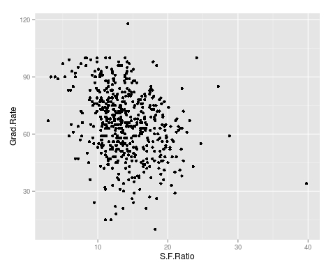
As you can see, there appears to be a negative relationship between student faculty ratio and grad rate. In other words, as the ration of student to faculty increases there is a decrease in the graduation rate.

Next, we will color the plots on the graph based on whether they are a public or private university to get a better understanding of the data. Below is the code for this followed by the plot.

> qplot(S.F.Ratio, Grad.Rate, colour = Private, data=trainingSet)
Rplot.jpeg
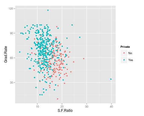
It appears that private colleges usually have lower student to faculty ratios and also higher graduation rates than public colleges

Add Regression Line

We will now plot the same data but will add a regression line. This will provide us with a visual of the slope. Below is the code followed by the plot.

> collegeplot<-qplot(S.F.Ratio, Grad.Rate, colour = Private, data=trainingSet) > collegeplot+geom_smooth(method = ‘lm’,formula=y~x)
Rplot01.jpeg
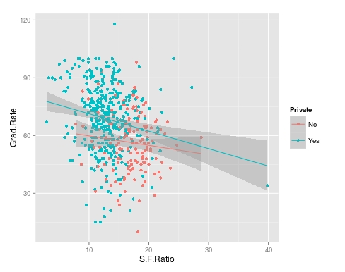
Most of this code should be familiar to you. We saved the plot as the variable ‘collegeplot’. In the second line of code, we add specific coding for ‘ggplot2’ to add the regression line. ‘lm’ means linear model and formula is for creating the regression.

Cutting the Data

We will now divide the data based on the student-faculty ratio into three equal size groups to look for additional trends. To do this you need the “Hmisc” packaged. Below is the code followed by the table

> library(Hmisc)
> divide_College<-cut2(trainingSet$S.F.Ratio, g=3)
> table(divide_College)
divide_College
[ 2.9,12.3) [12.3,15.2) [15.2,39.8] 
        185         179         181

Our data is now divided into three equal sizes.

Box Plots

Lastly, we will make a box plot with our three equal size groups based on student-faculty ratio. Below is the code followed by the box plot

CollegeBP<-qplot(divide_College, Grad.Rate, data=trainingSet, fill=divide_College, geom=c(“boxplot”)) > CollegeBP
Rplot02
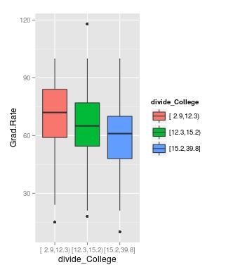
As you can see, the negative relationship continues even when student-faculty is divided into three equally size groups. However, our information about private and public college is missing. To fix this we need to make a table as shown in the code below.

> CollegeTable<-table(divide_College, trainingSet$Private)
> CollegeTable
              
divide_College  No Yes
   [ 2.9,12.3)  14 171
   [12.3,15.2)  27 152
   [15.2,39.8] 106  75

This table tells you how many public and private colleges there based on the division of the student-faculty ratio into three groups. We can also get proportions by using the following

> prop.table(CollegeTable, 1)
              
divide_College         No        Yes
   [ 2.9,12.3) 0.07567568 0.92432432
   [12.3,15.2) 0.15083799 0.84916201
   [15.2,39.8] 0.58563536 0.41436464

In this post, we found that there is a negative relationship between student-faculty ratio and graduation rate. We also found that private colleges have a lower student-faculty ratio and a higher graduation rate than public colleges. In other words, the status of a university as public or private moderates the relationship between student-faculty ratio and graduation rate.

You can probably tell by now that R can be a lot of fun with some basic knowledge of coding.

Thinking Skills

Everybody thinks, at least we hope everybody thinks. However, few are aware of the various skills that can be used in thinking. In this post, we will look at several different skills that can be used when trying to think and understand something. There are at least four different skills that can be used in thinking and they are…

  • Clarification
  • Basis
  • Inference
  • Evaluation

Clarification

Clarification, as you can tell from the name, is focused on making things clear so that decisions can be made. Clarification involves developing questions, analysis, and defining terms.

Clarification lays the groundwork for determining the boundaries in which thinking needs to take place. In many ways, clarification deals with the question of what are you trying to think about.

Basis

Basis involves categorizing the information that has been gathered to think about. At this stage, a person decides if the information they have is a fact, opinion, or just incorrect information.

Another activity at this level is assessing the credibility of the sources of information. For example, facts from experts are considered more credible than the opinions of just anybody.

Inference

Inference involves several different forms of reasoning. These forms of reasoning have been discussed in a previous post. The forms include inductive, deductive, and abductive reasoning.

Whatever form of reasoning is used the overall goal is to develop conclusions based either on principles or examples. As such, the prior forms of thinking are necessary to move to developing inferences. In other words, there must be clarification and basis before inferences.

Evaluation

Evaluation involves developing a criteria upon which to judge the adequacy of whatever decisions have been made. This means assessing the quality of the thought process that has already taken place.

Assessing judgment is near the top of Bloom’s Taxonomy and involves not only having an opinion but basing the opinion on well-developed criteria. This is in no way easy for anybody.

Tips for Developing Thinking Skills

When dealing with students, here are a few suggestions for developing thinking skills.

  • Demonstrate-Providing examples of the thinking process give students something to model.
  • Question-Questioning is an excellent way to develop thinking. Most of the thinking skills above involve extensive questioning.
  • Verbalize thinking-When students are required to think, have them verbalize what they are thinking. This provides insight into what is happening inside their head as well as allows the teacher to analyze what is happening.

Conclusion

Thinking involves questioning. The development of answers to these questions is the fruit of thinking. It is important to determine what one is trying to do in order to allow purposeful thinking to take place.

Grounded Theory: Emerging & Constructivist Design

Grounded theory is a qualitative methodology that was described briefly in this blog previously when we looked at systematic design. In this post, we will look at two other designs that fall under the grounded theory approach which are emerging and constructivist design.

Emerging Design

Emerging design was in many ways a reaction to systematic design. Glaser and Strauss worked together to develop grounded theory during the 1960’s. By the 1990’s Strauss along with Corbin had refined grounded theory into what is now know as systematic design.

Glasser had issues with systematic design. He considered it too rigid and strict with the emphasis on rules and procedures. In response to this, he developed the emerging design.

Glasser proposed to allow the theory to emerge from the data rather than forcing the data into preconceived categories. Glasser was also focused on a more iterative approach. This means that data was compared to data, data was compared to category, and category compared to category.

Glasser viewed grounded theory as the process of abstracting to higher and higher level rather than only describing a process. The generate theory should appropriately fit the data, should actually work, be relevant, and changeable.

Constructivist Design

The constructivist design is the youngest of the three grounded theory designs. It was first developed in the earlier 2000’s by Charmaz. Unlike the other forms of grounded theory with the focus on categories, codes, and theory generating. The constructivist design emphasizes the views, values, and feelings of the people rather than the process.

Whereas Strauss & Corbin and Glasser would focus on describing a process in their systematic or emerging design approach, the constructivist design would focus on how people felt during these process and try to extract meaning from the experience.

For example, if we conducted a study on men with chronic illness the results would vary depending on the grounded theory design we used. If we used systematic or emerging design we would focus on the common process of acquiring and dealing with a chronic illness. However, if we used the constructivist design we would focus on how the men feel during their experience with a chronic illness as well as trying to determine what it means to have a chronic illness.

Which to Choose?

The decision of what design is best depends on the purpose of the study and the preference of the researcher. It is difficult to say one is better or worst than the other. Rather, each is appropriate depending on the context of the study.

Predicting with Caret

In this post, we will explore the use of the caret package for developing algorithms for use in machine learning. The caret package is particularly useful for processing data before the actual analysis of the algorithm.

When developing algorithms is common practice to divide the data into a training a testing subsamples. The training subsample is what is used to develop the algorithm while the testing sample is used to assess the predictive power of the algorithm. There are many different ways to divide a sample into a testing and training set and one of the main benefits of the “caret” package is in dividing the sample.

In the example we will use, we will return to the “kearnlab” example and this develop an algorithm after sub-setting the sample to have a training data set and a testing data set.

First, you need to download the ‘caret’ and ‘kearnlab’ package if you have not done so. After that below is the code for subsetting the ‘spam’ data from the ‘kearnlab’ package.

inTrain<- createDataPartition(y=spam$type, p=0.75, 
list=FALSE)
training<-spam[inTrain,]
testing<-spam[-inTrain,] 
dim(training)

Here is what we did

  1. We created the variable ‘inTrain’
  2. In the variable ‘inTrain’ we told R to make a partition in the data use the ‘createDataPartition’ function. I the parenthesis we told r to look at the dataset ‘spam’ and to examine the variable ‘type’. Then we told are to pull 75% of the data in ‘type’ and copy it to the ‘inTrain’ variable we created. List = False tells R not to make a list. If you look closely, you will see that the variable ‘type’ is being set as the y variable in the ‘inTrain’ data set. This means that all the other variables in the data set will be used as predictors. Also, remember that the ‘type’ variable has two outcomes “spam” or “nonspam”
  3. Next, we created the variable ‘training’ which is the dataset we will use for developing our algorithm. To make this we take the original ‘spam’ data and subset the ‘inTrain’ partition. Now all the data that is in the ‘inTrain’ partition is now in the ‘training’ variable.
  4. Finally, we create the ‘testing’ variable which will be used for testing the algorithm. To make this variable, we tell R to take everything that was not assigned to the ‘inTrain’ variable and put it into the ‘testing’ variable. This is done through the use of a negative sign
  5. The ‘dim’ function just tells us how many rows and columns we have as shown below.
[1] 3451   58

As you can see, we have 3451 rows and 58 columns. Rows are for different observations and columns are for the variables in the data set.

Now to make the model. We are going to bootstrap our sample. Bootstrapping involves random sampling from the sample with replacement in order to assess the stability of the results. Below is the code for the bootstrap and model development followed by an explanation.

set.seed(32343)
SpamModel<-train(type ~., data=training, method="glm")
SpamModel

Here is what we did,

  1. Whenever you bootstrap, it is wise to set the seed. This allows you to reproduce the same results each time. For us, we set the seed to 32343
  2. Next, we developed the actual model. We gave the model the name “SpamModel” we used the ‘train’ function. Inside the parenthesis, we tell r to set “type” as the y variable and then use ~. which is a shorthand for using all other variables in the model as predictor variables. Then we set the data to the ‘training’ data set and indicate that the method is ‘glm’ which means generalized linear model.
  3. The output for the analysis is available at the link SpamModel

There is a lot of information but the most important information for us is the accuracy of the model which is 91.3%. The kappa stat tells us what the expected accuracy of the model is which is 81.7%. This means that our model is a little bit better than the expected accuracy.

For our final trick, we will develop a confusion matrix to assess the accuracy of our model using the ‘testing’ sample we made earlier. Below is the code

SpamPredict<-predict(SpamModel, newdata=testing)
confusionMatrix(SpamPredict, testing$type)

Here is what we did,

  1. We made a variable called ‘SpamPredict’. We use the function ‘predict’ using the ‘SpamModel’ with the new data called ‘testing’.
  2. Next, we make matrix using the ‘confusionMatrix’ function using the new model ‘SpamPredict’ based on the ‘testing’ data on the ‘type’ variable. Below is the output

Reference

  1. Prediction nonspam spam
       nonspam     657   35
       spam         40  418
                                              
                   Accuracy : 0.9348          
                     95% CI : (0.9189, 0.9484)
        No Information Rate : 0.6061          
        P-Value [Acc > NIR] : <2e-16          
                                              
                      Kappa : 0.8637          
     Mcnemar's Test P-Value : 0.6442          
                                              
                Sensitivity : 0.9426          
                Specificity : 0.9227          
             Pos Pred Value : 0.9494          
             Neg Pred Value : 0.9127          
                 Prevalence : 0.6061          
             Detection Rate : 0.5713          
       Detection Prevalence : 0.6017          
          Balanced Accuracy : 0.9327          
                                              
           'Positive' Class : nonspam

    The accuracy of the model actually improved to 93% on the test data. The other values such as sensitivity and specificity have to do with such things as looking at correct classifications divided by false negatives and other technical matters. As you can see, machine learning is a somewhat complex experience

Reasoning

Reasoning is the process of developing conclusion through the examination of evidence. This post will explain several forms of reasoning as listed below.

  • Inductive
  • Deductive
  • Causal
  • Analogical
  • Abductive

Inductive Reasoning

Inductive reasoning involves looking at several specific instances or facts and developing a conclusion. Below is an example

  • Fact 1: Dad died from smoking
  • Fact 2: Grandpa died from smoking
  • Fact 3: Uncle is dying from smoking
  • Conclusion: Smoking kills

In the example above, there are several instances of the effect of smoking on people. From these examples, the conclusion reach was smoking is deadly.

The danger of this form of reasoning is jumping to conclusions based on a small sample size. Just because three people died or are dying of smoking does not mean that smoking is deadly in general. This is not enough evidence to support this conclusion

Deductive Reasoning 

Deductive reasoning involves the development of a general principle testing a specific example of the principle and moving to a  conclusion. Below is an example.

  • Principle: Everybody is mortal
  • Specific example: Thomas is a man
  • Conclusion: Therefore, Thomas is mortal

This method of reasoning is highly effective in persuasion. However, the principle must be sound in order to impact the audience.

Causal Reasoning

Causal reasoning attempts to establish a relationship between a cause and effect. An example would be as follows.

You slip and break your leg. After breaking your leg you notice that there was a banana on the ground. You therefore reason that you slipped on the banana and broke your leg

The danger of causal reasoning is it is sometimes difficult to prove cause and effect conclusively. In addition, complex events cannot often be explained by a single cause.

Analogical Reasoning

Analogical reasoning involves the comparison of two similar cases making the argument that what is true for the first is true for the second. Below is an example.

  • Fact 1: Thomas is good at playing the trumpet
  • Fact 2: Thomas is good at playing the French Horn
  • Conclusion: Thomas is probably good at playing the trombone

The example above assumes that Thomas can play the trombone because he can play other brass instruments well. It is critical that the comparison made is truly parallel in order to persuade an audience.

Abductive Reasoning

Abductive reasoning involves looking at incomplete information and trying to make sense of this through reasonable guesses. Perhaps the most common experiences people have with abductive reasoning is going to the hospital or mechanic. In both situations, the doctor and mechanic listen to the symptoms and try to make a diagnosis as to exactly what the problem is.

Of course, the doctor and mechanic can be completely wrong which leads to other problems. However, unlike the other forms of reasoning, abductive reasoning is useful for filling in gaps in information that is unavailable.

Conclusion

Reasoning comes in many forms. The examples provided here provide people with different ways these forms of reasoning can be used.