Monthly Archives: May 2016

ARCS Model of Motivational Design

The ARCS model of motivational design is an instructional model used in education. Instructional models are used to facilitate the learning experience of students. The ARCS model provides a step-by-step process of engaging students, building there confidence, and providing a sense of satisfaction during a learning experience.

In this post, we will look at the various aspects of the ARCS model as they are based on the acronym below

A  ttention
R  elevance
C  onfidence
S  atisfaction

A-ttention

Attention is the first step in the ARCS model. The goal at this stage is to help the learner to focus on the lesson.  There are several different ways to do this and they include the following.

  • Examples such as stories, and or audiovisual.
  • Hands-on experience such as experiments, skits, etc
  • Incongruity and Conflict which can be through employing cognitive dissonance. For example, making a statement that confuses students could provide a hook to get them to focus on the lesson
  • Inquiry involves having students ask questions to pull them into the lesson. The questions they develop rouse their desire to find the answer

None of these approaches are exclusive, which means that they can be used in combination with each other. For example, you could use an example to cause incongruity and or inquiry. The point is that a teacher must find a way to get their students’ attention.

R-elevance

Relevance is about using concepts and ideas the students can connect with to explain whatever new ideas are in the lesson. If students can see how what they are learning connect with their lives they are more inclined to learn it. Below are some ways to bring relevance into a lesson

  • Future usefulness means showing the students how what they are learning will help them later. This is not the strongest approach but it provides a platform for developing relevancy.
  • Needs matching means helping students to discover that they need to learn a particular skill or idea. When students know they need to learn something they are often motivated to learn it.
  • Modeling means being an example for the students. By demonstrating the new skill, student have something that they can imitate. This relates well with social learning theory.
  • Choice is highly motivating for many students. Through empowering students, there is often an increase in making learning relevant.

C-onfidence

Developing confidence is about providing students with opportunities to succeed. What this means for the teacher is to provide assessment and activities that are stimulating but not impossible to complete.

A general rule of thumb is that students should be a able to successful complete 60-70% of a new skill on the first try. This allows them to have some degree of success while still indicating where they need to improve.

S-atisfaction

Satisfaction is closely related to confidence. With satisfaction, you provide the students with authentic situation in which to use their newly acquire skills. This implies the use of authentic assessments. However, authentic assessment requires feedback in order for the student to understand their growth opportunities.

Conclusion

The ARCS model provides teachers with an easy to follow template for developing clear instruction. The foundational principles in this model are useful for anyone who is looking for a way to vary their teaching practices.

The Natural Approach to Language Acquisition

The Natural Approach is a somewhat radical approach in language teaching. By radical I mean that it was often anti-everything that was happening in language teaching at the time of its development. Now, the Natural Approach is considered a fringe but not too shocking in terms of the philosophy behind it.

In this post, we will look at the assumptions, curriculum and of the Natural Approach

Assumptions

The Natural Approach is based on cognitivism and starts with the assumption that language learning emerges naturally if students are given appropriate exposure and conditions.

The focus is always upon the meaning of words and grammar is not focused upon. There is no need to explicitly analyze the grammatical structure of a language. Instead, the Natural Approach, students need time to develop gradually a knowledge of the rules. The language experience must always be slightly beyond the student’s ability as this stretches the student to continue to grow.

The Natural Approach also encourages maintaining an enjoyable and warm classroom environment. This is believed to help with motivation, self-confidence, and anxiety.

Curriculum

The Natural Approach is intended for beginners in a language. Therefore, the most basic skills are acquired from the use of this approach. The learner plays a role in the development of the curriculum. They are expected to do the following.

  • Share their goals for learning the language
  • Deciding when they want to begin to talk in the target language
  • Make sure the communication in the class is comprehensible

The teacher’s role is to provide clear examples of the target language. The teacher is also expected to provide a friendly warm atmosphere of learning. Lastly, the teacher needs to provide a variety of learning experiences.

The teacher achieves these goals through the use of games and group activities. Singing is another aspect of the Natural Approach as well. Basically, the students experience the language in a fun, low-stress environment. Through this easy-going experience, language acquisition takes place.

Conclusion

The Natural Approach to language learning is distinct in its cognitive focused yet relax environment emphasis. This approach is highly useful for training children in particular in acquiring a new language as the focus is more on fun than the academic discipline of learning.

Making a Decision Tree in R

In this post, we are going to learn how to use the C5.0 algorithm to make a classification tree in order to make predictions about gender based on wage, education, and job experience using a data set in the “Ecdat” package in R. Below is some code to get started.

library(Ecdat); library(C50); library(gmodels)
 data(Wages1)

We now will explore the data to get a sense of what is happening in it. Below is the code for this

str(Wages1)
 ## 'data.frame': 3294 obs. of 4 variables:
 ## $ exper : int 9 12 11 9 8 9 8 10 12 7 ...
 ## $ sex : Factor w/ 2 levels "female","male": 1 1 1 1 1 1 1 1 1 1 ...
 ## $ school: int 13 12 11 14 14 14 12 12 10 12 ...
 ## $ wage : num 6.32 5.48 3.64 4.59 2.42 ...
 hist(Wages1$exper)

Rplot02

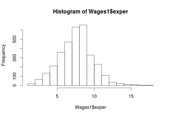
summary(Wages1$exper)
 ## Min. 1st Qu. Median Mean 3rd Qu. Max.
 ## 1.000 7.000 8.000 8.043 9.000 18.000

hist(Wages1$wage)

Rplot

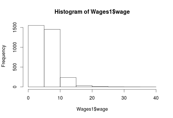
summary(Wages1$wage)
## Min. 1st Qu. Median Mean 3rd Qu. Max.
## 0.07656 3.62200 5.20600 5.75800 7.30500 39.81000

hist(Wages1$school)

Rplot01

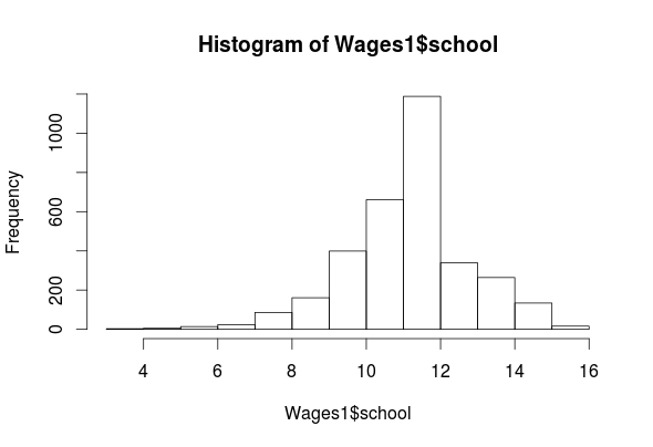
summary(Wages1$school)
 ## Min. 1st Qu. Median Mean 3rd Qu. Max.
 ## 3.00 11.00 12.00 11.63 12.00 16.00

table(Wages1$sex)
## female male
## 1569 1725

As you can see, we have four features (exper, sex, school, wage) in the “Wages1” data set. The histogram for “exper” indicates that it is normally distributed. The “wage” feature is highly left-skewed and almost bimodal. This is not a big deal as classification trees are robust against non-normality. The ‘school’ feature is mostly normally distributed. Lastly, the ‘sex’ feature is categorical but there is almost an equal number of men and women in the data. All of the outputs for the means are listed above.

Create Training and Testing Sets

We now need to create our training and testing data sets. In order to do this, we need to first randomly reorder our data set. For example, if the data is sorted by one of the features, to split it now would lead to extreme values all being lumped together in one data set.

To make things more confusing, we also need to set our seed. This allows us to be able to replicate our results. Below is the code for doing this.

set.seed(12345)
 Wage_rand<-Wages1[order(runif(3294)),]

What we did is explained as follows

  1. set the seed using the ‘set.seed’ function (We randomly picked the number 12345)
  2. We created the variable ‘Wage_rand’ and we assigned the following
  3. From the ‘Wages1’ dataset we used the ‘runif’ function to create a list of 3294 numbers (1-3294) we did this because there are a total of 3294 examples in the dataset.
  4. After generating the 3294 numbers we then order sequentially using the “order” function.
  5. We then assigned each example in the “Wages1” dataset one of the numbers we created

We will now create are training and testing set using the code below.

Wage_train<-Wage_rand[1:2294,]
 Wage_test<-Wage_rand[2295:3294,]

Make the Model
We can now begin training a model below is the code.

Wage_model<-C5.0(Wage_train[-2], Wage_train$sex)

The coding for making the model should be familiar by now. One thing that is new is the brackets with the -2 inside. This tells r to ignore the second column in the dataset. We are doing this because we want to predict sex. If it is a part of the independent variables we cannot predict it. We can now examine the results of our model by using the following code.

Wage_model
##
## Call:
## C5.0.default(x = Wage_train[-2], y = Wage_train$sex)
##
## Classification Tree
## Number of samples: 2294
## Number of predictors: 3
##
## Tree size: 9
##
## Non-standard options: attempt to group attributes
summary(Wage_model)
##
## Call:
## C5.0.default(x = Wage_train[-2], y = Wage_train$sex)
##
##
## C5.0 [Release 2.07 GPL Edition] Wed May 25 10:55:22 2016
## ——————————-
##
## Class specified by attribute `outcome’
##
## Read 2294 cases (4 attributes) from undefined.data
##
## Decision tree:
##
## wage <= 3.985179: ## :…school > 11: female (345/109)
## : school <= 11:
## : :…exper <= 8: female (224/96) ## : exper > 8: male (143/59)
## wage > 3.985179:
## :…wage > 9.478313: male (254/61)
## wage <= 9.478313: ## :…school > 12: female (320/132)
## school <= 12:
## :…school <= 10: male (246/70) ## school > 10:
## :…school <= 11: male (265/114) ## school > 11:
## :…exper <= 6: female (83/35) ## exper > 6: male (414/173)
##
##
## Evaluation on training data (2294 cases):
##
## Decision Tree
## —————-
## Size Errors
##
## 9 849(37.0%) <<
##
##
## (a) (b) ## —- —-
## 600 477 (a): class female
## 372 845 (b): class male
##
##
## Attribute usage:
##
## 100.00% wage
## 88.93% school
## 37.66% exper
##
##
## Time: 0.0 secs

The “Wage_model” indicates a small decision tree of only 9 decisions. The “summary” function shows the actual decision tree. It’s somewhat complicated but I will explain the beginning part of the tree.

If wages are less than or equal to 3.98 then the person is female THEN

If the school is greater than 11 then the person is female ELSE

If the school is less than or equal to 11 THEN

If The experience of the person is less than or equal to 8 the person is female ELSE

If the experience is greater than 8 the person is male etc.

The next part of the output shows the amount of error. This model misclassified 37% of the examples which is pretty high. 477 men were misclassified as women and 372 women were misclassified as men.

Predict with the Model

We will now see how well this model predicts gender in the testing set. Below is the code

Wage_pred<-predict(Wage_model, Wage_test)

CrossTable(Wage_test$sex, Wage_pred, prop.c = FALSE,
 prop.r = FALSE, dnn=c('actual sex', 'predicted sex'))

The output will not display properly here. Please see C50 for a pdf of this post and go to page 7

Again, this code should be mostly familiar for the prediction model. For the table, we are comparing the test set sex with predicted sex. The overall model was correct 269 + 346/1000 for 61.5% accuracy rate, which is pretty bad.

Improve the Model

There are two ways we are going to try and improve our model. The first is adaptive boosting and the second is error cost.

Adaptive boosting involves making several models that “vote” how to classify an example. To do this you need to add the ‘trials’ parameter to the code. The ‘trial’ parameter sets the upper limit of the number of models R will iterate if necessary. Below is the code for this and the code for the results.

Wage_boost10<-C5.0(Wage_train[-2], Wage_train$sex, trials = 10)
 #view boosted model
 summary(Wage_boost10)
 ##
 ## Call:
 ## C5.0.default(x = Wage_train[-2], y = Wage_train$sex, trials = 10)
 ##
 ##
 ## C5.0 [Release 2.07 GPL Edition] Wed May 25 10:55:22 2016
 ## -------------------------------
 ##
 ## Class specified by attribute `outcome'
 ##
 ## Read 2294 cases (4 attributes) from undefined.data
 ##
 ## ----- Trial 0: -----
 ##
 ## Decision tree:
 ##
 ## wage <= 3.985179: ## :...school > 11: female (345/109)
 ## : school <= 11:
 ## : :...exper <= 8: female (224/96) ## : exper > 8: male (143/59)
 ## wage > 3.985179:
 ## :...wage > 9.478313: male (254/61)
 ## wage <= 9.478313: ## :...school > 12: female (320/132)
 ## school <= 12:
 ## :...school <= 10: male (246/70) ## school > 10:
 ## :...school <= 11: male (265/114) ## school > 11:
 ## :...exper <= 6: female (83/35) ## exper > 6: male (414/173)
 ##
 ## ----- Trial 1: -----
 ##
 ## Decision tree:
 ##
 ## wage > 6.848846: male (663.6/245)
 ## wage <= 6.848846:
 ## :...school <= 10: male (413.9/175) ## school > 10: female (1216.5/537.6)
 ##
 ## ----- Trial 2: -----
 ##
 ## Decision tree:
 ##
 ## wage <= 3.234474: female (458.1/192.9) ## wage > 3.234474: male (1835.9/826.2)
 ##
 ## ----- Trial 3: -----
 ##
 ## Decision tree:
 ##
 ## wage > 9.478313: male (234.8/82.1)
 ## wage <= 9.478313:
 ## :...school <= 11: male (883.2/417.8) ## school > 11: female (1175.9/545.1)
 ##
 ## ----- Trial 4: -----
 ##
 ## Decision tree:
 ## male (2294/1128.1)
 ##
 ## *** boosting reduced to 4 trials since last classifier is very inaccurate
 ##
 ##
 ## Evaluation on training data (2294 cases):
 ##
 ## Trial Decision Tree
 ## ----- ----------------
 ## Size Errors
 ##
 ## 0 9 849(37.0%)
 ## 1 3 917(40.0%)
 ## 2 2 958(41.8%)
 ## 3 3 949(41.4%)
 ## boost 864(37.7%) <<
 ##
 ##
 ## (a) (b) ## ---- ----
 ## 507 570 (a): class female
 ## 294 923 (b): class male
 ##
 ##
 ## Attribute usage:
 ##
 ## 100.00% wage
 ## 88.93% school
 ## 37.66% exper
 ##
 ##
 ## Time: 0.0 secs

R only created 4 models as there was no additional improvement after this. You can see each model in the printout. The overall results are similar to our original model that was not boosted. We will now see how well our boosted model predicts with the code below.

Wage_boost_pred10<-predict(Wage_boost10, Wage_test)
 CrossTable(Wage_test$sex, Wage_boost_pred10, prop.c = FALSE,
 prop.r = FALSE, dnn=c('actual Sex Boost', 'predicted Sex Boost'))

Our boosted model has an accuracy rate 223+379/1000 = 60.2% which is about 1% better then our unboosted model (59.1%). As such, boosting the model was not useful (see page 11 of the pdf for the table printout.)

Our next effort will be through the use of a cost matrix. A cost matrix allows you to impose a penalty on false positives and negatives at your discretion. This is useful if certain mistakes are too costly for the learner to make. IN our example, we are going to make it 4 times more costly misclassify a female as a male (false negative) and 1 times for costly to misclassify a male as a female (false positive). Below is the code

error_cost Wage_cost<-C5.0(Wage_train[-21], Wage_train$sex, cost = error_cost)
 Wage_cost_pred<-predict(Wage_cost, Wage_test)
 CrossTable(Wage_test$sex, Wage_cost_pred, prop.c = FALSE,
 prop.r = FALSE, dnn=c('actual Sex EC', 'predicted Sex EC'))

With this small change our model is 100% accurate (see page 12 of the pdf).

Conclusion

This post provided an example of decision trees. Such a model allows someone to predict a given outcome when given specific information.

Understanding Decision Trees

Decision trees are yet another method of machine learning that is used for classifying outcomes. Decision trees are very useful for, as you can guess, making decisions based on the characteristics of the data.

In this post, we will discuss the following

  • Physical traits of decision trees
  • How decision trees work
  • Pros and cons of decision trees

Physical Traits of a Decision Tree

Decision trees consist of what is called a tree structure. The tree structure consists of a root node, decision nodes, branches and leaf nodes.

A root node is an initial decision made in the tree. This depends on which feature the algorithm selects first.

Following the root node, the tree splits into various branches. Each branch leads to an additional decision node where the data is further subdivided. When you reach the bottom of a tree at the terminal node(s) these are also called leaf nodes.

How Decision Trees Work

Decision trees use a heuristic called recursive partitioning. What this does is it splits the overall dataset into smaller and smaller subsets until each subset is as close to pure (having the same characteristics) as possible. This process is also known as divide and conquer.

The mathematics for deciding how to split the data is based on an equation called entropy, which measures the purity of a potential decision node. The lower the entropy scores the purer the decision node is. The entropy can range from 0 (most pure) to 1 (most impure).

One of the most popular algorithms for developing decision trees is the C5.0 algorithm. This algorithm, in particular, uses entropy to assess potential decision nodes.

Pros and Cons

The prose of decision trees includes its versatile nature. Decision trees can deal with all types of data as well as missing data. Furthermore, this approach learns automatically and only uses the most important features. Lastly, a deep understanding of mathematics is not necessary to use this method in comparison to more complex models.

Some problems with decision trees are that they can easily overfit the data. This means that the tree does not generalize well to other datasets. In addition, a large complex tree can be hard to interpret, which may be yet another indication of overfitting.

Conclusion

Decision trees provide another vehicle that researchers can use to empower decision making. This model is most useful particularly when a decision that was made needs to be explained and defended. For example, when rejecting a person’s loan application. Complex models made provide stronger mathematical reasons but would be difficult to explain to an irate customer.

Therefore, for complex calculation presented in an easy to follow format. Decision trees are one possibility.

Types of Mixed Method Design

In a previous post, we looked at mix methods and some examples of this design. Mixed methods are focused on combining quantitative and qualitative methods to study a research problem. In this post, we will look at several additional mixed method designs. Specifically, we will look at the follow designs

  • Embedded design
  • Transformative design
  • Multi-phase design

Embedded Design

Embedded design is the simultaneous collection of quantitative and qualitative data with one form of data by supportive to the other. The supportive data augments the conclusions of the main data collection.

The benefits of this design is that allows for one method to lead the analysis with the secondary method provides additional information. For example, quantitative measures are excellent at recording the results of an experiment. Qualitative measures would be useful in determining how participants perceived their experience in the experiment.

A downside to this approach making sure the secondary method is truly supporting the overall research. Quantitative and qualitative methods natural answer different research questions. Therefore, the research questions of a study must be worded in a way that allows for cooperation between qualitative and quantitative methods.

Transformative Design

The transformative design is more of a philosophy than a mixed method design. This design can employ any other mixed method design. The main difference that transformative designs focus on helping a marginalized population with the goal of bringing about change.

For example, a researcher might do a study Asian students facing discrimination in a predominately African American high school. The goal of the study would be to document the experiences of Asian students in order to provide administrators with information on the extent of this problem.

Such a focus on the oppressed is drawn heavily from Critical Theory which exposes how oppression takes place through education. The emphasis on change is derived from Dewy and progressivism.

Multiphase Design

Multiphase design is actually the use of several designs over several studies. This is a massive and supremely complex process. You would need to tie together several different mixed method studies under one general research problem. From this, you can see that this is not a commonly used design.

For example, you may decide to continue doing research into Asian student discrimination at African American high schools. The first study might employ an explanatory design. The second study might employ and exploratory design. The last study might be a transformative design.

After completing all this work, you would need to be able to articulate the experiences with discrimination of the Asian students. This is not an easy task by any means. As such, if and when this design is used, it often requires the teamwork of several researchers.

Conclusion

Mixed method designs require a different way of thinking when it comes to research. The uniqueness of this approach is the combination of qualitative and quantitative methods. This mixing of methods has advantages and disadvantage. The primary point to remember is that the most appropriate design depends on the circumstances of the study.

Cooperative Language Learning

Cooperative language learning (CLL) is the application of the instructional method cooperative learning in the language classroom. This approach to language teaching was a reaction against the teacher-centered methods of its time in favor of learner-centered methods.

This post will discuss the assumptions of CLL as well as the instructional practices associated with it.

Assumptions

Proponents of CLL see language as a primary tool for social interactions. Students learn the language through these social interactions. This idea is based primarily upon the work of Vygotsky. In addition, language also serves the function of communication and accomplishing tasks. This implies a need for authentic assessment.

The student’s role is to work as a member of a group. CLL questions if learning a language alone is an appropriate way to learn. The teacher must provide a highly structured environment in which they serve as a facilitator of learning.

Curriculum 

CLL has several specific goals including the following.

  • Learn the target language naturally through group interaction
  • Develop learning strategies
  • Create a positive learning environment
  • Develop critical thinking skills

These goals are partially achieved through developing interdependence among the students, individual accountability, and the formation of groups. Interdependence is useful in showing students that what benefits one benefits all of them.

Individual accountability happens through not only assigning group grades but individual grades as well for projects. Lastly, group formation is the foundation of the CLL experience.

Some common activities based on CLL includes

  • Jigsaw-Divide the work and then have the students put the pieces together
  • Projects-Any assignment that requires more than one person
  • Think-Pair-Share-Pose a question, let them think, put them in pairs, and have each pair share.

All of these activities involve collaboration with communication in the target language.

Conclusion

CLL involves learning in groups rather than alone. There is research that indicates that CLL is beneficial in acquiring the target language. As such, CLL is yet another way in which language teachers can support their students.

Conditional Probability & Bayes’ Theorem

In a prior post, we look at some of the basics of probability. The prior forms of probability we looked at focused on independent events, which are events that are unrelated to each other.

In this post, we will look at conditional probability which involves calculating probabilities for events that are dependent on each other. We will understand conditional probability through the use of Bayes’ theorem.

Conditional Probability 

If all events were independent of it would be impossible to predict anything because there would be no relationships between features. However, there are many examples of on event affecting another. For example, thunder and lighting can be used to predictors of rain and lack of study can be used as a predictor of test performance.

Thomas Bayes develop a theorem to understand conditional probability. A theorem is a statement that can be proven true through the use of math. Bayes’ theorem is written as follows

P(A | B)

This complex notation simply means

The probability of event A given event B occurs

Calculating probabilities using Bayes’ theorem can be somewhat confusing when done by hand. There are a few terms however that you need to be exposed too.

  • prior probability is the probability of an event without a conditional event
  • likelihood is the probability of a given event
  • posterior probability is the probability of an event given that another event occurred. the calculation or posterior probability is the application of Bayes’ theorem

Naive Bayes Algorithm

Bayes’ theorem has been used to develop the Naive Bayes Algorithm. This algorithm is particularly useful in classifying text data, such as emails. This algorithm is fast, good with missing data, and powerful with large or small data sets. However, naive Bayes struggles with large amounts of numeric data and it has a problem with assuming that all features are of equal value, which is rarely the case.

Conclusion

Probability is a core component of prediction. However, prediction cannot truly take place with events being dependent. Thanks to the work of Thomas Bayes, we have one approach to making prediction through the use of his theorem.

In a future post, we will use naive Bayes algorithm to make predictions about text.

Introduction to Probability

Probability is a critical component of statistical analysis and serves as a way to determine the likelihood of an event occurring. This post will provide a brief introduction into some of the principles of probability.

Probability 

There are several basic probability terms we need to cover

  • events
  • trial
  • mutually exclusive and exhaustive

Events are possible outcomes. For example, if you flip a coin, the event can be heads or tails. A trial is a single opportunity for an event to occur. For example, if you flip a coin one time this means that there was one trial or one opportunity for the event of heads or tails to occur.

To calculate the probability of an event you need to take the number of trials an event occurred divided by the total number of trials. The capital letter “P” followed by the number in parentheses is always how probability is expressed. Below is the actual equation for this

Number of trial the event occurredTotal number of trials = P(event)

To provide an example, if we flip a coin ten times and we recored five heads and five tails, if we want to know the probability of heads this is the answer below

Five heads ⁄ Ten trials = P(heads) = 0.5

Another term to understand is mutually exclusive and exhaustive. This means that events cannot occur at the same time. For example, if we flip a coin, the result can only be heads or tails. We cannot flip a coin and have both heads and tails happen simultaneously.

Joint Probability 

There are times were events are not mutually exclusive. For example, lets say we have the possible events

  1. Musicians
  2. Female
  3.  Female musicians

There are many different events that came happen simultaneously

  • Someone is a musician and not female
  • Someone who is female and not a musician
  • Someone who is a female musician

There are also other things we need to keep in mind

  • Everyone is not female
  • Everyone is not a musician
  • There are many people who are not female and are not musicians

We can now work through a sample problem as shown below.

25% of the population are musicians and 60% of the population is female. What is the probability that someone is a female musician

To solve this problem we need to find the joint probability which is the probability of two independent events happening at the same time. Independent events or events that do not influence each other. For example, being female has no influence on becoming a musician and vice versa. For our female musician example, we run the follow calculation.

P(Being Musician) * P(Being Female) = 0.25 * 0.60 = 0.25 = 15%

 From the calculation, we can see that there is a 15% chance that someone will be female and a musician.

Conclusion

Probability is the foundation of statistical inference. We will see in a future post that not all events are independent. When they are not the use of conditional probability and Bayes theorem is appropriate.

Mixed Methods

Mix Methods research involves the combination of qualitative and quantitative approaches to addressing a research problem. Generally, qualitative and quantitative methods have separate philosophical positions when it comes to how to uncover insights in addressing research questions.

For many, mixed methods have their own philosophical position, which is pragmatism. Pragmatists believe that if it works it’s good. Therefore, if mixed methods lead to a solution it’s an appropriate method to use.

This post will try to explain some of the mixed method designs. Before explaining it is important to understand that there are several common ways to approach mixed methods

  • Qualitative and Quantitative are equal (Convergent Parallel Design)
  • Quantitative is more important than qualitative (explanatory design)
  • Qualitative is more important than quantitative

Convergent Parallel Design 

This design involves the simultaneous collecting of qualitative and quantitative data. The results are then compared to provide insights into the problem. The advantage of this design is the quantitative data provides for generalizability while the qualitative data provides information about the context of the study.

However, the challenge is in trying to merge the two types of data. Qualitative and quantitative methods answer slightly different questions about a problem. As such it can be difficult to paint a picture of the results that are comprehensible.

Explanatory Design

This design puts emphasis on the quantitative data with qualitative data playing a secondary role. Normally, the results found in the quantitative data are followed up on in the qualitative part.

For example, if you collect surveys about what students think about college and the results indicate negative opinions, you might conduct an interview with students to understand why they are negative towards college. A Likert survey will not explain why students are negative. Interviews will help to capture why students have a particular position.

The advantage of this approach is the clear organization of the data. Quantitative data is more important. The drawback is deciding what about the quantitative data to explore when conducting the qualitative data collection.

Exploratory Design 

This design is the opposite of explanatory. Now the qualitative data is more important than the quantitative. This design is used when you want to understand a phenomenon in order to measure it.

It is common when developing an instrument to interview people in focus groups to understand the phenomenon. For example, if I want to understand what cellphone addiction is I might ask students to share what they think about this in interviews. From there, I could develop a survey instrument to measure cell phone addiction.

The drawback to this approach is the time consumption. It takes a lot of work to conduct interviews, develop an instrument, and assess the instrument.

Conclusions

Mixed methods are not that new. However, they are still a somewhat unusual approach to research in many fields. Despite this, the approaches of mixed methods can be beneficial depending on the context.

Lexical Approach

The Lexical Approach is a unique approach in TESOL methods. This approach starts from the position that language learning is not about the individual word but rather multi-word chunks. As such, a student should focus learning various combinations of word chunks.

This post will share the assumptions and curriculum of the Lexical Approach

Assumptions

The Lexical Approach states clearly that language acquisition happens through acquiring the chunks or collocations of a language. Learning a language is not about rules but rather about acquiring enough examples from which the learner can make generalizations. For example, I child will eventually learn that “good morning” is a greeting for a  specific time of day.

Chunks are learned through one or more of the following strategies

  • Exposure-You see it over and over again and make a generalization
  • Comparison-You compare the target language chunk with a chunk for another language
  • Noticing-You notice a combination for the first time

Lexical approach is primarily an approach for developing autonomous learning. Therefore, the teacher’s role is to provide an environment in which the student can manage their own learning.

The student’s responsibility is in using what is called a concordancer. A concordancer is an online resource that provides examples of how a word is used in real literature. Each concordancer has one or more corpus from which examples of the word being used come from.

Curriculum

The Lexical Approach is not a comprehensive method and as such does not include any objectives. There are several common activities used in this approach.

  • Awareness activities help students to notice chunks and include. The teacher might provide several examples of sentences using the word “prediction” to allow students to try and determine the meaning of this word
  • Identifying chunks involves having the students search for chunks in a text. The results are then compared during a discussion.
  • Retelling involves having a student make their own sentences while reusing a chunk that they have just learned. For example, if the students learn the chunk (don’t put all your eggs in one basket) they would have to use this chunk in their own unique sentence.

Conclusion

The Lexical approach is a useful approach for those with a more analytical way of learning a language. Digesting a language through memorizing and applying various collocations can be beneficial to many language learners.

Nearest Neighbor Classification in R

In this post, we will conduct a nearest neighbor classification using R. In a previous post, we discussed nearest neighbor classification. To summarize, nearest neighbor uses the traits of a known example to classify an unknown example. The classification is determined by the closets known example(s) to the unknown example. There are essentially four steps in order to complete a nearest neighbor classification

  1. Find a dataset
  2. Explore/prepare the Dataset
  3. Train the model
  4. Evaluate the model

For this example, we will use the college data set from the ISLR package. Our goal will be to predict which colleges are private or not private based on the feature “Private”. Below is the code for this.

library(ISLR)
 data("College")

Step 2 Exploring the Data

We now need to explore and prep the data for analysis. Exploration helps us to find any problems in the data set. Below is the code, you can see the results in your own computer if you are following along.

str(College)
prop.table(table(College$Private))
summary(College)

The “str” function gave us an understanding of the different types of variables and some of there initial values. We have 18 variables in all. We want to predict “Private” which is a categorical feature Nearest neighbor predicts categorical features only. We will use all of the other numerical variables to predict “Private”. The prop.table give us the proportion of private and not private colleges. About 30% of the data is not private and about 70% is a private college

Lastly, the “summary” function gives us some descriptive stats. If you look closely at the descriptive stats, there is a problem. The variables use different scales. For example, the “Apps” feature goes from 81 to 48094 while the “Grad.Rate” feature goes from 10 to 100. If we do the analysis with these different scales the “App” feature will be a much stronger influence on the prediction. Therefore, we need to rescale the features or normalize them. Below is the code to do this

 normal<-function(x){
 return((x-min(x))/(max(x)))
 }

We made a function called “normal” that normalizes or scales are variables so that all values are between 0-1. This makes all of the features equal in their influence. We now run code to normalize our data using the “normal” function we created. We will also look at the summary stats. In addition, we will leave out the prediction feature “Private” because we do not want to have that in the new data set because we want to predict this. In a real-world example, you would not know this before the analysis anyway.

College_New<-as.data.frame(lapply(College[2:18],normal))
summary(College_New)

The name of the new dataset is “College_New” we used the “lapply” function to make R normalize all the features in the “College” dataset. Summary stats are good as all values are between 0 and 1. The last part of this step involves dividing our data into training and testing sets as seen in the code below and creating the labels. The labels are the actual information from the “Private” feature. Remember, we remove this from the “College_New” dataset but we need to put this information in their own features to allow us to check the accuracy of our results later.

College_train<-College_New[1:677, ]
 College_Test<-College_New[678:777,]
 #make labels
 College_train_labels<-College[1:677, 1]
 College_test_labels<-College[678:777,1]

Step 3 Model Training

Train the model We will now train the model. You will need to download the “class” package and load it. After that, you need to run the following code.

library(class)
 College_test_pred<-knn(train=College_train, test=College_Test,
 cl=College_train_labels, k=25)

Here is what we did

  • We created a variable called “College_test_pred” to store our results
  • We used the “knn” function to predict the examples. Inside the “knn” function we used “College_train” to teach the model.
  • We then identify “College_test” as the dataset we want to test. For the ‘cl’ argument we used the “College_train_labels” dataset which contains which colleges are private in the “College_train” dataset. The “k” is the number of neighbors that knn uses to determine what class to label an unknown example. In this code, we are using the 25 nearest neighbors to label the unknown example The number of “k” to use can vary but a rule of thumb is to take the square root of the total number of examples in the training data. Our training data has 677 and the square root of this is about 25. What happens is that each of the 25 closest neighbors are calculated for an example. If 20 are not private and 5 are private the unknown example is labeled private because the majority of its neighbors are not private.

Step 4 Evaluating the Model

We will now evaluate the model using the following code

 library(gmodels)
 CrossTable(x=College_test_labels, y=College_test_pred, prop.chisq = FALSE)

The results can be seen by clicking here.  The box in the top left predicts which colleges are private correctly while the box in the bottom right classifies which colleges are not private correctly. For example, 28 colleges that are not private were classed as not private while 64 colleges that are not private were classed as not private. Adding these two numbers together gives us 92 (28+64) which is our accuracy rate. In the top right box, we have are false positives. These are colleges which are private but were predicted as private, there were 8 of these. Lastly, we have our false negatives in the bottom left box, which are colleges that are private but label as not private, there were 0 of these.

Conclusion

The results are pretty good for this example. Nearest neighbor classification allows you to predict an unknown example based on the classification of the known neighbors. This is a simple way to identify examples that are clump among neighbors with the same characteristics.

Text-Based Instruction

Text-Based Instruction (TBI) employs the use of different genres of text in a social context to encourage language development. This post will discuss the assumptions and curriculum development of this method.

Assumptions

TBI starts with the belief that different forms of text are used for various situations. This leads to another conclusion that mastering a language involves exposure to these different genres.  Furthermore, each text has a distinct organizational pattern

However, exposure to different types of text is not enough. Students must also use language in a social setting. Communicating about the text is critical for language acquisition.

TBI also stresses the importance of learning explicitly about the language. This means conscious awareness about what one is learning. This again can happen through discussion or through the illustrations of the teacher. In fact, scaffolding is a key component of TBI.

Students learn through the guidance and support of the teacher. The teacher’s role, in addition to scaffolding, is to select materials and sequence the curriculum.

Curriculum

The objectives in a TBI curriculum depends on the text that is used in the learning experiences. For example, the objectives for reading newspapers are different from reading textbooks.

Instructional materials play a crucial role in TBI. This is because of the emphasis on authentic materials. As such, actual reading samples from books, articles, and magazines are commonly employed.

A common instructional approach using TBI would include the following steps

  1. Build the context
    • This means providing a background about the reading through sharing necessary information for an understanding of the topic of the text. This can be done verbally, visually, a combination of both, etc.
  2. Deonstructing the text
    • This involves comparing the writing of the text the students are using with another similarly written text. For example, comparing the structure of to newspaper articles.
  3. Joint Construction of text
    • Students, with the support of the teacher, develop their own example of the text they were reading. For example, if the text was a newspaper article. The class develops a sample newspaper article with teacher support.
  4. Independent construction of text
    • Same as #3 but now the students work alone.
  5. Reflection
    • Students discuss how what they learned can be used in other contexts

Conclusion

TBI is a unique approach to language teaching that focuses on reading to develop the other three skills of language. This approach is particularly useful for people who prefer to learn a language through reading rather than in other forms.

Characteristics of Big Data

In a previous post, we talked about types of Big Data. However, another way to look at big data and define it is by looking at the characteristics of Big Data. In other words, what helps to identify makes Big Data as data that is big.

This post will explain the 6 main characteristics of Big Data. These characteristics are often known as the V’s of Big Data. They are as follows

  • Volume
  • Variety
  • Velocity
  • Veracity
  • Valence
  • Value

Volume

Volume has to do with the size of the data. It is hard to comprehend how volume is measured in computer science when it comes to memory for many people. Most of the computers that the average person uses works in the range of gigabytes. For example, a dvd will hold about 5 gigabytes of data.

It is now becoming more and more common to find people with terabytes of storage. A terabyte is 1,000 gigabytes! This is enough memory to hold 500 dvds worth of data. The next step up is petabytes which is 1000 terabytes or 5,000,000 dvds.

Big data involves data that is large as in the examples above. Such massive amounts of data called on new ways of analysis.

Variety

Variety is another term for complexity. Big data can be highly or lowly complex. There was a previous post about structured and unstructured data that we won’t repeat here. The point is that these various levels of complexity make analysis highly difficult because of the tremendous amount of data mugging or cleaning of the data that is often necessary.

Velocity

Velocity is the speed at which big data is created, stored, and or analyzed. Two approaches to processing data are batch and real-time. Batch processing involves collecting and cleaning the data in “batches” for processing. It is necessary to wait for all the “batches” to come in before making a decision. As such this is a slow process.

An alternative is real-team processing. This approach involves streaming the information into machines which process the data immediately.

The speed at which data needs to be processed is linked directly with the cost. As such, faster may not always be better or necessary.

Veracity

The quality of the data is what veracity is. If the data is no good the results are no good. The most reliable data tends to be collected companies and other forms of enterprise. The next lower level is social media data. Finally, the lowest level of data is often data that is captured by sensors. The differences between the levels is often the lack of discrimination.

Valence

Valence is a term that is used in chemistry and has to do with how an element has electrons available for bonding with other elements. This can lead to complex molecules due to elements being interconnected through sharing electrons.

In Big Data, valence is how interconnected the data is. As there are more and more connections among the data the complexity of the analysis increases.

Value

Value is the ability to convert Big Data information into a monetary reward. For example, if you find a relationship between two products at a point of sale, you can recommend them to customers at a website or put the products next to each in a store.

A lot of Big Data research is done with a motive of making money. However, there is a lot of Big Data research happening that is driven exclusively by a profit motive such as the research being used to analyze the human genome. As such, the “value” characteristic is not always included when talking about the characteristics of Big Data.

Conclusion

Understanding the traits of Big Data allows an individual to identify Big Data when they see it. The traits here are the common ones of Big Data. However, this list is far from exhaustive and there is much more that could be said.