
In this post, we will conduct a logistic regression analysis. Logistic regression is used when you want to predict a categorical dependent variable using continuous or categorical dependent variables. In our example, we want to predict Sex (male or female) when using several continuous variables from the “survey” dataset in the “MASS” package.

library(MASS);library(bestglm);library(reshape2);library(corrplot)data(survey)
?MASS::survey #explains the variables in the studyThe first thing we need to do is remove the independent factor variables from our dataset. The reason for this is that the function that we will use for the cross-validation does not accept factors. We will first use the “str” function to identify factor variables and then remove them from the dataset. We also need to remove in examples that are missing data so we use the “na.omit” function for this. Below is the code
survey$Clap<-NULL
survey$W.Hnd<-NULL
survey$Fold<-NULL
survey$Exer<-NULL
survey$Smoke<-NULL
survey$M.I<-NULL
survey<-na.omit(survey)
We now need to check for collinearity using the “corrplot.mixed” function form the “corrplot” package.
pc<-cor(survey[,2:5])
corrplot.mixed(pc)
corrplot.mixed(pc)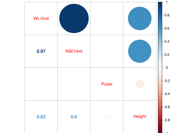
We have an extreme correlation between “We.Hnd” and “NW.Hnd” this makes sense because people’s hands are normally the same size. Since this blog post is a demonstration of logistic regression we will not worry about this too much.
We now need to divide our dataset into a train and a test set. We set the seed for. First, we need to make a variable that we call “ind” that is randomly assigned 70% of the number of rows of survey 1 and 30% 2. We then subset the “train” dataset by taking all rows that are 1’s based on the “ind” variable and we create the “test” dataset for all the rows that line up with 2 in the “ind” variable. This means our data split is 70% train and 30% test. Below is the code
set.seed(123)
ind<-sample(2,nrow(survey),replace=T,prob = c(0.7,0.3))
train<-survey[ind==1,]
test<-survey[ind==2,]
We now make our model. We use the “glm” function for logistic regression. We set the family argument to “binomial”. Next, we look at the results as well as the odds ratios.
fit<-glm(Sex~.,family=binomial,train)
summary(fit)
##
## Call:
## glm(formula = Sex ~ ., family = binomial, data = train)
##
## Deviance Residuals:
## Min 1Q Median 3Q Max
## -1.9875 -0.5466 -0.1395 0.3834 3.4443
##
## Coefficients:
## Estimate Std. Error z value Pr(>|z|)
## (Intercept) -46.42175 8.74961 -5.306 1.12e-07 ***
## Wr.Hnd -0.43499 0.66357 -0.656 0.512
## NW.Hnd 1.05633 0.70034 1.508 0.131
## Pulse -0.02406 0.02356 -1.021 0.307
## Height 0.21062 0.05208 4.044 5.26e-05 ***
## Age 0.00894 0.05368 0.167 0.868
## ---
## Signif. codes: 0 '***' 0.001 '**' 0.01 '*' 0.05 '.' 0.1 ' ' 1
##
## (Dispersion parameter for binomial family taken to be 1)
##
## Null deviance: 169.14 on 122 degrees of freedom
## Residual deviance: 81.15 on 117 degrees of freedom
## AIC: 93.15
##
## Number of Fisher Scoring iterations: 6exp(coef(fit))## (Intercept) Wr.Hnd NW.Hnd Pulse Height
## 6.907034e-21 6.472741e-01 2.875803e+00 9.762315e-01 1.234447e+00
## Age
## 1.008980e+00The results indicate that only height is useful in predicting if someone is a male or female. The second piece of code shares the odds ratios. The odds ratio tell how a one unit increase in the independent variable leads to an increase in the odds of being male in our model. For example, for every one unit increase in height there is a 1.23 increase in the odds of a particular example being male.
We now need to see how well our model does on the train and test dataset. We first capture the probabilities and save them to the train dataset as “probs”. Next we create a “predict” variable and place the string “Female” in the same number of rows as are in the “train” dataset. Then we rewrite the “predict” variable by changing any example that has a probability above 0.5 as “Male”. Then we make a table of our results to see the number correct, false positives/negatives. Lastly, we calculate the accuracy rate. Below is the code.
train$probs<-predict(fit, type = 'response')
train$predict<-rep('Female',123)
train$predict[train$probs>0.5]<-"Male"
table(train$predict,train$Sex)
##
## Female Male
## Female 61 7
## Male 7 48mean(train$predict==train$Sex)## [1] 0.8861789Despite the weaknesses of the model with so many insignificant variables it is surprisingly accurate at 88.6%. Let’s see how well we do on the “test” dataset.
test$prob<-predict(fit,newdata = test, type = 'response')
test$predict<-rep('Female',46)
test$predict[test$prob>0.5]<-"Male"
table(test$predict,test$Sex)
##
## Female Male
## Female 17 3
## Male 0 26mean(test$predict==test$Sex)## [1] 0.9347826As you can see, we do even better on the test set with an accuracy of 93.4%. Our model is looking pretty good and height is an excellent predictor of sex which makes complete sense. However, in the next post we will use cross-validation and the ROC plot to further assess the quality of it.