In this post, we will learn how to do exploratory work to determine where fraud is in a dataset. Such knowledge can be used to inform the development of a model.

Libraries

Below are the libraries we are using. The setup is simple.

import pandas as pd
import matplotlib.pyplot as plt

No data preparation is required in this analysis. Therefore, we will proceed to the exploratory process. What we will do is examine the data and drop the useless variable, as shown below.

df=df.drop('Unnamed: 0', axis=1)
print(df.head())

  age gender           category  amount  fraud
0   3      F  es_transportation   49.71      0
1   4      F          es_health   39.29      0
2   3      F  es_transportation   18.76      0
3   4      M  es_transportation   13.95      0
4   2      M  es_transportation   49.87      0

We will now examine fraud by groups

Find Fraud by Groups

We will start by filtering for only data that is considered fraud.

# Create two dataframes with fraud and non-fraud data 
df_fraud = df.loc[df.fraud == 1] 
df_non_fraud = df.loc[df.fraud == 0]

We will be pulling from the df_fraud dataset and the df dataset for the rest of this post. We will group our data according to category, age, and gender.

The code finding fraud by group is complicated, but here is what we are doing.

1. In the first part of the code. We found the total amount of money spent without considering fraud.
2. Part 2: We find the percent of fraud
3. Part 3: We calculate the average amount of fraud when there is an instance of fraud
4. Part 4: We calculate the total instances by category
5. Part 5: We change the column order and sort values

Below is the code and output

#Fraud by category
category_fraud=df_fraud.groupby('category').sum('amount').sort_values(['fraud','amount'],ascending=False)

#average amount and percent of fraud to non-fraud
category_fraud[['avg_amount','fraud_per']]=df.groupby('category').mean('fraud')

#average amount of fraud
category_fraud['average_fraud']=category_fraud['amount']/category_fraud['fraud']

#Examples by category
category_fraud['n']=df['category'].value_counts()

#Change column order and sort values 
category_fraud=category_fraud.reindex(columns=['n','fraud','fraud_per','average_fraud','amount','avg_amount'])
category_fraud=category_fraud.sort_values(['fraud_per','fraud'],ascending=False)

print(category_fraud)

What we learn from this is the following

• Every instance of es_leisure is fraud
• Almost every instance of es_travel is fraud
• the majority of es_sportsandtoys, es_otherservices, and es_hotel_services
• Not all categories have instances of fraud. We will not determine their names for the sake of time.

We will now repeat this process for age and gender

age_fraud=df_fraud.groupby('age').sum('amount')
age_fraud[['avg_amount','fraud_per']]=df.groupby('age').mean('fraud')
age_fraud['average_fraud']=age_fraud['amount']/age_fraud['fraud']
age_fraud['n']=df['age'].value_counts()
age_fraud=age_fraud.reindex(columns=['n','fraud','fraud_per','average_fraud','amount','avg_amount'])
age_fraud=age_fraud.sort_values(['fraud_per','fraud'],ascending=False)
print(age_fraud)

        n  fraud  fraud_per  average_fraud      amount  avg_amount
age                                                               
0      40      2   0.050000     210.473700    420.9474   49.468935
4    1279     46   0.035966     165.624843   7618.7428   36.197985
2    2333     67   0.028718     190.049045  12733.2860   37.228665
1     713     19   0.026648     191.477305   3638.0688   35.622829
5     792     19   0.023990     184.388358   3503.3788   37.547521
3    1718     40   0.023283     210.251670   8410.0668   37.279338
6     314      7   0.022293     186.037086   1302.2596   36.700852

The main points are

• Fraud is an anomaly across the age categories

Lastly, gender

gender_fraud=df_fraud.groupby('gender').sum('amount')
gender_fraud[['avg_amount','fraud_per']]=df.groupby('gender').mean('fraud')
gender_fraud['average_fraud']=gender_fraud['amount']/gender_fraud['fraud']
gender_fraud['n']=df['gender'].value_counts()
gender_fraud=gender_fraud.reindex(columns=['n','fraud','fraud_per','average_fraud','amount','avg_amount'])
gender_fraud=gender_fraud.sort_values(['fraud_per','fraud'],ascending=False)
print(gender_fraud)

           n  fraud  fraud_per  average_fraud      amount  avg_amount
gender                                                               
F       3972    133   0.033484     186.432140  24795.4746   37.842941
M       3212     67   0.020859     191.511576  12831.2756   35.918978

As with age, fraud is an anomaly.

Another point is that the average_fraud is around 180-190 for all groups.

Visual

Below, we will make a histogram comparing the distribution of fraud amounts to non-fraud amounts

# Plot histograms of the amounts in fraud and non-fraud data 
plt.hist(df_fraud.amount, alpha=0.5, label='fraud')
plt.hist(df_non_fraud.amount, alpha=0.5, label='nonfraud')
plt.legend()
plt.show()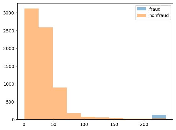

As you can see, the fraud values are a little over 200. This information can be used to set up a model for detecting fraud.

Conclusion

Data exploration is a powerful tool to determine the steps to take in developing your model. These insights help to provide focus in model development and provide you with an understanding of the traits and characteristics of your data. Understanding your data not only helps with model development but also with creating justifications for the approach that is taken.