In this post, we will learn how to do exploratory work to determine where fraud is in a dataset. Such knowledge can be used to inform the development of a model.

Libraries

Below are the libraries we are using. The setup is simple.

import pandas as pd
import matplotlib.pyplot as plt

No data preparation is required in this analysis. Therefore, we will proceed to the exploratory process. What we will do is examine the data and drop the useless variable, as shown below.

df=df.drop('Unnamed: 0', axis=1)
print(df.head())

  age gender           category  amount  fraud
0   3      F  es_transportation   49.71      0
1   4      F          es_health   39.29      0
2   3      F  es_transportation   18.76      0
3   4      M  es_transportation   13.95      0
4   2      M  es_transportation   49.87      0

We will now examine fraud by groups

Find Fraud by Groups

We will start by filtering for only data that is considered fraud.

# Create two dataframes with fraud and non-fraud data 
df_fraud = df.loc[df.fraud == 1] 
df_non_fraud = df.loc[df.fraud == 0]

We will be pulling from the df_fraud dataset and the df dataset for the rest of this post. We will group our data according to category, age, and gender.

The code finding fraud by group is complicated, but here is what we are doing.

1. In the first part of the code. We found the total amount of money spent without considering fraud.
2. Part 2: We find the percent of fraud
3. Part 3: We calculate the average amount of fraud when there is an instance of fraud
4. Part 4: We calculate the total instances by category
5. Part 5: We change the column order and sort values

Below is the code and output

#Fraud by category
category_fraud=df_fraud.groupby('category').sum('amount').sort_values(['fraud','amount'],ascending=False)

#average amount and percent of fraud to non-fraud
category_fraud[['avg_amount','fraud_per']]=df.groupby('category').mean('fraud')

#average amount of fraud
category_fraud['average_fraud']=category_fraud['amount']/category_fraud['fraud']

#Examples by category
category_fraud['n']=df['category'].value_counts()

#Change column order and sort values 
category_fraud=category_fraud.reindex(columns=['n','fraud','fraud_per','average_fraud','amount','avg_amount'])
category_fraud=category_fraud.sort_values(['fraud_per','fraud'],ascending=False)

print(category_fraud)

What we learn from this is the following

• Every instance of es_leisure is fraud
• Almost every instance of es_travel is fraud
• the majority of es_sportsandtoys, es_otherservices, and es_hotel_services
• Not all categories have instances of fraud. We will not determine their names for the sake of time.

We will now repeat this process for age and gender

age_fraud=df_fraud.groupby('age').sum('amount')
age_fraud[['avg_amount','fraud_per']]=df.groupby('age').mean('fraud')
age_fraud['average_fraud']=age_fraud['amount']/age_fraud['fraud']
age_fraud['n']=df['age'].value_counts()
age_fraud=age_fraud.reindex(columns=['n','fraud','fraud_per','average_fraud','amount','avg_amount'])
age_fraud=age_fraud.sort_values(['fraud_per','fraud'],ascending=False)
print(age_fraud)

        n  fraud  fraud_per  average_fraud      amount  avg_amount
age                                                               
0      40      2   0.050000     210.473700    420.9474   49.468935
4    1279     46   0.035966     165.624843   7618.7428   36.197985
2    2333     67   0.028718     190.049045  12733.2860   37.228665
1     713     19   0.026648     191.477305   3638.0688   35.622829
5     792     19   0.023990     184.388358   3503.3788   37.547521
3    1718     40   0.023283     210.251670   8410.0668   37.279338
6     314      7   0.022293     186.037086   1302.2596   36.700852

The main points are

• Fraud is an anomaly across the age categories

Lastly, gender

gender_fraud=df_fraud.groupby('gender').sum('amount')
gender_fraud[['avg_amount','fraud_per']]=df.groupby('gender').mean('fraud')
gender_fraud['average_fraud']=gender_fraud['amount']/gender_fraud['fraud']
gender_fraud['n']=df['gender'].value_counts()
gender_fraud=gender_fraud.reindex(columns=['n','fraud','fraud_per','average_fraud','amount','avg_amount'])
gender_fraud=gender_fraud.sort_values(['fraud_per','fraud'],ascending=False)
print(gender_fraud)

           n  fraud  fraud_per  average_fraud      amount  avg_amount
gender                                                               
F       3972    133   0.033484     186.432140  24795.4746   37.842941
M       3212     67   0.020859     191.511576  12831.2756   35.918978

As with age, fraud is an anomaly.

Another point is that the average_fraud is around 180-190 for all groups.

Visual

Below, we will make a histogram comparing the distribution of fraud amounts to non-fraud amounts

# Plot histograms of the amounts in fraud and non-fraud data 
plt.hist(df_fraud.amount, alpha=0.5, label='fraud')
plt.hist(df_non_fraud.amount, alpha=0.5, label='nonfraud')
plt.legend()
plt.show()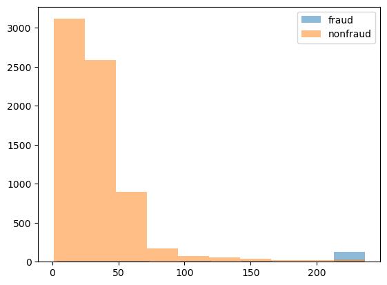

As you can see, the fraud values are a little over 200. This information can be used to set up a model for detecting fraud.

Conclusion

Data exploration is a powerful tool to determine the steps to take in developing your model. These insights help to provide focus in model development and provide you with an understanding of the traits and characteristics of your data. Understanding your data not only helps with model development but also with creating justifications for the approach that is taken.

Ensemble methods enable the use of multiple algorithms to make predictions. Instead of only random forest or logistic regression, you can use both, and the results from each model can be used in a “vote” to make predictions. This is one way to combine the strengths of various models to make stronger predictions

Libraries

Below are the libraries that we are using. We are using three different algorithms for our ensemble (random forest, logistic regression, and decision trees). A new function we are using is the VotingClassifer() function, which is used to create our ensemble model. The other functions have been used and explained previously.

from sklearn.linear_model import LogisticRegression
from sklearn.ensemble import VotingClassifier
from sklearn.ensemble import RandomForestClassifier
from sklearn.tree import DecisionTreeClassifier
from sklearn.model_selection import train_test_split
from sklearn.metrics import confusion_matrix, classification_report, roc_auc_score
from sklearn.model_selection import GridSearchCV
import pandas as pd
import numpy as np
df = pd.read_csv("C:/Users/dthom/Documents/python/fraud/chapter_2/chapter_2/creditcard_sampledata_2.csv")

We will now proceed to the data preparation.

Data Prep

The data preparation is simple. We will separate the independent variables from the dependent variables. The X object represents all of the independent variables, while the y object represents our dependent variable, fraud or no fraud. Once everything is separated, we will create our train and test sets using the train_test_split() function. 70% of our data will be used for training, and 30% will be used for testing.

X = df.iloc[:, 1:30]    
X = np.array(X).astype('float')    
y = df.iloc[:, 30]    
y=np.array(y).astype('float')

# Split your data into training and test set
X_train, X_test, y_train, y_test = train_test_split(X, y, test_size=.3, random_state=0)

The next step will involve creating our initial ensemble model.

Model Development

We will use three different classifiers in our ensemble model. The classifiers are logistic regression, random forest, and decision tree. In the code below, each classifier is called, and we also set the various parameters of each classifier to appropriate initial values.

# Define the three classifiers to use in the ensemble
clf1 = LogisticRegression(class_weight={0:1, 1:15},max_iter=1000, random_state=5)
clf2 = RandomForestClassifier(class_weight={0:1, 1:12}, criterion='gini', max_depth=8, max_features='log2',
            min_samples_leaf=10, n_estimators=30, n_jobs=-1, random_state=5)
clf3 = DecisionTreeClassifier(random_state=5, class_weight="balanced")

We will now combine all of our different models into a single model using the VotingClassifier() function. The estimators are given names in quotes, followed by the object after a comma. The “voting” parameter is set to “hard.” Hard voting allows for each model to get one vote per case, with the simple majority winning. For example, if logistic regression and random forest predict fraud simple majority wins this case.

Once we create our combined model, we also fit our data and make predictions. This will allow us to determine the strength of our model.

# Combine the classifiers in the ensemble model
ensemble_model = VotingClassifier(estimators=[('lr', clf1), ('rf', clf2), ('dt', clf3)], voting='hard') #define  voting
ensemble_model.fit(X_train, y_train)
predicted = ensemble_model.predict(X_test) #no probabilities with voting

Next, we will assess the initial results

Model Assessment

In the code below, we use the classification_report() function and confusion_matrix() to see our results.

print(classification_report(y_test, predicted))
print(confusion_matrix(y_test, predicted))

              precision    recall  f1-score   support

         0.0       0.99      1.00      0.99      2099
         1.0       0.89      0.86      0.87        91

    accuracy                           0.99      2190
   macro avg       0.94      0.93      0.93      2190
weighted avg       0.99      0.99      0.99      2190

[[2089   10]
 [  13   78]]

The strength of this model depends on its goals and how it compares to other models. For practice, we will modify the model below.

Model Modification

We will not make any changes to the individual models. Instead, we will make some adjustments to the ensemble model. IN the code below, we are changing the voting to “soft,” which means we are using the probabilities to predict rather than a majority vote. The weights are set so that the second model (random forest) has 4 times the influence compared to the other models. Lastly, the flatten_transform argument is related to the voting argument and changes the output of the data. Below is the code

#Change the weight of the models
# Define the ensemble model
ensemble_model = VotingClassifier(estimators=[('lr', clf1), ('rf', clf2), ('dt', clf3)], 
                                 voting='soft', 
                                 weights=[1, 4, 1], 
                                 flatten_transform=True)

We will now fit our data and predict with it

ensemble_model.fit(X_train, y_train)
predicted = ensemble_model.predict(X_test) #no probabilities with voting

Next, we assess the model

Model Assessment

The model is mostly the same, with a slight improvement in precision. In other words, false positives were reduced.

print(classification_report(y_test, predicted))
print(confusion_matrix(y_test, predicted))

              precision    recall  f1-score   support

         0.0       0.99      1.00      1.00      2099
         1.0       0.94      0.86      0.90        91

    accuracy                           0.99      2190
   macro avg       0.97      0.93      0.95      2190
weighted avg       0.99      0.99      0.99      2190

[[2094    5]
 [  13   78]]

Conclusion

In this post, we saw how models can work together to make stronger, more robust predictions. Ensemble methods are a powerful way to improve fraud detection, and you now know ways to modify the model.

In this post, we will utilize an algorithm that is slightly more sophisticated than the traditional approach of creating rules. We will use logistic regression to determine whether fraud has occurred or not. The details of how logistic regression works are beyond the scope of this post. However, you can find information on logistic regression here.

Libraries

We will begin by loading our libraries and preparing the data

import pandas as pd
import numpy as np
from sklearn.linear_model import LogisticRegression
from sklearn.model_selection import train_test_split
from sklearn.metrics import confusion_matrix
from sklearn.metrics import classification_report

df = pd.read_csv(df_loc)

Pandas and numpy are for data preparation. The rest of the libraries are self-explanatory. LogisticRegression is for logistic regression. train_test_split is for creating our train and test sets. The last two libraries provide tools for assessing our model. The last line of code loads our data. This data is not available on the internet.

Data Preparation

Below, we take a look at the data.

df.head()
Out[5]: 
   Unnamed: 0        V1        V2        V3        V4        V5        V6  \
0      258647  1.725265 -1.337256 -1.012687 -0.361656 -1.431611 -1.098681   
1       69263  0.683254 -1.681875  0.533349 -0.326064 -1.455603  0.101832   
2       96552  1.067973 -0.656667  1.029738  0.253899 -1.172715  0.073232   
3      281898  0.119513  0.729275 -1.678879 -1.551408  3.128914  3.210632   
4       86917  1.271253  0.275694  0.159568  1.003096 -0.128535 -0.608730   

There are more variables than this. Our goal is to predict fraud using the available variables. In the code below, we will separate the X and y values, which will be crucial when creating our training and testing data.

# Separate X, and y values
X = df.iloc[:, 1:30]    
X = np.array(X).astype('float')    
y = df.iloc[:, 30]    
y=np.array(y).astype('float')

In the code above, we instructed Python to use columns 2 to 29 as the X values and convert them into an array. We then instructed Python to extract column 30 and create a separate array.

Create Train and Test Sets

We will now separate our data into training and test sets. We will train the data on the training set and test it with the other set. Below is the code.

# Create the training and testing sets
X_train, X_test, y_train, y_test = train_test_split(X, y, test_size=.3, random_state=0)

In the code above, we create four objects, which are all to the left of the equal sign. To the right of the equal sign, we have our function train_test_split(). This function is using our X and y objects from the data preparation section and separating them at a ratio of 70/30. In other words, 70% of the X and y values are for training and 30% are for testing. This is why the test_size argument is set to 0.3. Lastly, the random_state argument determines the seed, allowing you to replicate your approach.

Fit the Model

We will now fit our data to the model. We will create an instance of the logistic regression algorithm and call it “model”. The max_iter argument is to make sure the model converges. Next, we use the .fit() method with our training data. Lastly, we make our predictions using the .predict() method with the testing data

# Fit a logistic regression model to our data
model = LogisticRegression(max_iter=1000)
model.fit(X_train, y_train)

# Obtain model predictions
predicted = model.predict(X_test)

Model Accuracy

The model accuracy is below. The results indicate that the model struggles more with false positives (2) compared to false negatives (1). Whether this is a good model or not depends on comparison to other models and the context of the project.

# Print the classifcation report and confusion matrix
print('Classification report:\n', classification_report(y_test,predicted))
conf_mat = confusion_matrix(y_true=y_test, y_pred=predicted)
print('Confusion matrix:\n', conf_mat)

Classification report:
               precision    recall  f1-score   support

         0.0       1.00      1.00      1.00      1503
         1.0       0.91      0.83      0.87        12

    accuracy                           1.00      1515
   macro avg       0.95      0.92      0.93      1515
weighted avg       1.00      1.00      1.00      1515

Confusion matrix:
 [[1502    1]
 [   2   10]]

Conclusion

Logistic regression is one of many great tools for fraud detection. Compared to other approaches, it is still somewhat simple, which is another major benefit of using it.

In this post, we will modify a model when trying to detect fraud. Most, if not all, machine learning algorithms have parameters that can be adjusted. Adjusting these parameters can potentially improve the accuracy of the model. Each algorithm also has different parameters that can be tuned. For our purposes, we will be using the random forest algorithm.

Libraries

Below are the libraries we will use in this post.

from sklearn.ensemble import RandomForestClassifier
from sklearn.model_selection import train_test_split
from sklearn.metrics import confusion_matrix, classification_report, roc_auc_score
import pandas as pd
import numpy as np
import matplotlib.pyplot as plt

The RandomForestClassifier() is the function to create an instance of the random forest algorithm. The train_test_split() function will be used for splitting our data into training and test sets. The confusion_matrix(), classification_report(), and roc_auc_score() functions will be used for assessing our model’s performance. Pandas and numpy are for data preparation. Lastly, matplotlib will be used in conjunction with the roc_auc_score(), which will be explained in detail later.

Data Preparation

Below is the data preparation. In this code, we are separating the independent variables from the dependent variable. Columns 2-29 will be used to predict column 30. Column 30 tells us if the example is fraudulent or not.

X = df.iloc[:, 1:30]    
X = np.array(X).astype('float')    
y = df.iloc[:, 30]    
y=np.array(y).astype('float')

For the X object above, we pull columns 2-29. Then we convert the X object to an array in the next line. We repeat this process for the y object, but we only pull column 30.

In the code below, we are now splitting our X and y objects into training and testing data. The training data teaches the algorithm, and you then assess your model by using the testing data.

# Split your data into training and test set
X_train, X_test, y_train, y_test = train_test_split(X, y, test_size=.3, random_state=0)

We create four objects to the left of the equal sign, two each for the X object and the y object. To the left of the equal sign, we use our train_test_split() function to divide the X and y objects. The argument test_size tells Python what proportion of the data should be used for the test data. For our example, 30% of the data is set aside for testing purposes.

Model Development

In the code below, we are going to create our initial model using random forest.

# Define the model with balanced subsample
model = RandomForestClassifier(class_weight='balanced_subsample', random_state=5)

# Fit your training model to your training set
model.fit(X_train, y_train)

Above, we create an object called “model” that contains an instance of the random forest algorithm. Inside the function, we set the argument class_weights to balanced_subsample. Setting the class weight to balanced is common in fraud detection because there is an imbalance in the classes, as fraud is highly uncommon. By setting the class weights to balance it so that misclassifications of fraud and non-fraud have the same penalty. Remember that by default, 95% percent of our data is not fraudulent without the use of a model. In addition, a balanced subsample is used when each tree is bootstrapped or not, based on the training data.

After addressing imbalances, we then fit our model and calculate the probabilities that each predicted example is correct. These probabilities will be useful in making the orc curve score.

# Obtain the predicted values and probabilities from the model 
predicted = model.predict(X_test)
probs = model.predict_proba(X_test)

Next, we will assess the original model

Model Assessment

The code below provides several metrics. The roc_auc_score calculates sensitivity (true positive rate) against its 1-specificity (false positive rate) and ranges in value from 0 to 1. The closer the value is to 1, the better. Other metrics we calculate include metrics related to the classification_report() function (precision, recall, f1-score, and accuracy) and the confiusion_matrix(), which creates a crosstab of the results.

# Print the roc_auc_score, the classification report and confusion matrix
print(roc_auc_score(y_test, probs[:,1]))
print(classification_report(y_test, predicted))
print(confusion_matrix(y_test, predicted))

0.9604599783256286
              precision    recall  f1-score   support

         0.0       0.99      1.00      1.00      2099
         1.0       0.99      0.81      0.89        91

    accuracy                           0.99      2190
   macro avg       0.99      0.91      0.94      2190
weighted avg       0.99      0.99      0.99      2190

[[2098    1]
 [  17   74]]

The ROC curve value is 0.96, which indicates a strong model as the value is close to 1. Precision is much stronger than recall, which means the model is better at avoiding false positives than it is at avoiding false negatives. The F1-score is a composite of precision and recall. Also note that model accuracy is 99%, which is expected when dealing with fraud detection.

Model Adjustment

The initial model looks rather good, but there is always a question as to whether we can improve the model. In the code below, we make the following modifications to our model.

• Bootstrap set to true: This means that each tree that is developed will be based on a subsample of the data that is resampled. Therefore, each tree is not developed from identical data.
• class_weight: Previously, the weights were balanced. The new setting indicates we are manually assigning a weight of 1 to class 0 and a weight of 12 to class 1, and this tells the RandomForestClassifier model to penalize misclassifications of class 1 twelve times more heavily than misclassifications of class 0.
• criterion=’entropy’: Entropy is a measure of the purity of each node. The less mixture within a node (fraud and non-fraud), the higher the purity.
• max_depth: How deep the truth is allowed to go. If this is not set, the tree will descend until the nodes are pure.
• min_samples_leaf: The minimum number of examples required to split a node.
• n_estimators: The number of trees to developed
• n_jobs: Affects processing power that is used
• random_state: Sets the seed

The rest of the code is a repeat of before

# Change the model options
model = RandomForestClassifier(bootstrap=True, class_weight={0:1, 1:12}, criterion='entropy',
			
			# Change depth of model
            max_depth=10,
		
			# Change the number of samples in leaf nodes
            min_samples_leaf=10, 

			# Change the number of trees to use
            n_estimators=20, n_jobs=-1, random_state=5)

# Fit your training model to your training set
model.fit(X_train, y_train)

# Obtain the predicted values and probabilities from the model 
predicted = model.predict(X_test)
probs = model.predict_proba(X_test)

We will now assess this model

2nd Assessment

Below is the code for the second assessment of the model. This code is the same as before.

# Print the roc_auc_score, the classification report and confusion matrix
print(roc_auc_score(y_test, probs[:,1]))
print(classification_report(y_test, predicted))
print(confusion_matrix(y_test, predicted))

0.9575150909119465
              precision    recall  f1-score   support

         0.0       0.99      1.00      1.00      2099
         1.0       0.94      0.84      0.88        91

    accuracy                           0.99      2190
   macro avg       0.97      0.92      0.94      2190
weighted avg       0.99      0.99      0.99      2190

[[2094    5]
 [  15   76]]

The model lacks improvement. We were able to decrease the number of false negatives by increasing the number of false positives. Whether this is better depends on the context and deciding if false negatives or false positives are more detrimental.

Conclusion

What we learned here is how to not only create a model and assess it, but also how to make modifications to the model in hopes of improving it. The power of machine learning can help you improve models to have more success in detecting fraud.

In this post, we are using logistic regression and the sampling technique of SMOTE to improve our model’s ability to detect fraud. SMOTE creates synthetic cases of actual fraud in order to balance out the number of true and false cases in the dataset. We will begin by loading our libraries

Libraries

The libraries we are using are below. As we use these libraries, they will be explained.

from imblearn.pipeline import Pipeline 
from imblearn.over_sampling import SMOTE
import pandas as pd
import numpy as np
import matplotlib.pyplot as plt
from sklearn.linear_model import LogisticRegression
from sklearn.model_selection import train_test_split
from sklearn.metrics import confusion_matrix
from sklearn.metrics import classification_report

Data Preparation

We load our data using the .read_csv() method from pandas. The object data_loc was created to store the location of the data on the computer. The data used in this example is not available. After loading the data, we use .shape to see how many columns and rows of data we have. The code and output are below

df = pd.read_csv(data_loc)
df.shape
(5050, 31)

You can see that we have 5050 rows of data and 31 columns of data. Next, we need to separate the X values from the y value. To do this, we will take columns 2 to 29 as X values and column 30 as the y value. The code below completes all of this for us.

X = df.iloc[:, 1:30]    
X = np.array(X).astype('float')    
y = df.iloc[:, 30]    
y=np.array(y).astype('float')

In the code below, we are creating our train and test sets. We are going to split our X and y objects so that 70% of the data is for training and 30% of the data is for testing purposes. The function train_test_split() is used for this, with the argument test_size being set to 0.3 for 30% test data and the random_state being set to 0, which is the seed number.

# Split your data X and y, into a training and a test set and fit the pipeline onto the training data
X_train, X_test, y_train, y_test = train_test_split(X, y, test_size=.3, random_state=0)

Pipeline Development

A pipeline is used to chain several actions together sequentially and is similar to piping in R. To do this, we are using the Pipeline() function from the imblearn library. The imblearn library is used to address imbalances in datasets, as our data has. We will complete the pipeline by first creating an instance of SMOTE and logistic regression. We do this because these are the two objects we will pipe one after the other.

Next, we will actually create our pipe. We created an object called “pipeline” and used the Pipeline function. Inside this function are two tuples. The first is for SMOTE and uses the first object we create at the beginning of this cell, and the second contains the information of the object we created. Also, notice how both tuples are wrapped inside square brackets. The code for all of this is below

# Define which resampling method and which ML model to use in the pipeline
resampling = SMOTE()
model = LogisticRegression(max_iter=1000)

# Define the pipeline, tell it to combine SMOTE with the Logistic Regression model
pipeline = Pipeline([('SMOTE', resampling), ('Logistic Regression',model)])

What we did in this code was tell Python to use SMOTE to create synthetic cases of instances of fraud. Once the resampling is completed, the resampled data will be used to train the model.

Model Development and Performance Metrics

We will now train our model with the SMOTE data using logistic regression and make the predictions. We use the .fit() method with the pipeline object and then use the .predict() method with the test data. The code is below

# Fit your pipeline onto your training set and obtain predictions by fitting the model onto the test data 
pipeline.fit(X_train, y_train) 
predicted = pipeline.predict(X_test)

Now we run our performance metrics to see how our model did. We will use the classification_report() and confusion_matrix() functions. The classification_report function tells us the precision, recall, and f1-score. The confusion_metrix() function is a printout of a crosstab of our data. Notice in both of these metrics, we are using the y test values compared to the predicted values.

# Obtain the results from the classification report and confusion matrix 
print('Classifcation report:\n', classification_report(y_test, predicted))
conf_mat = confusion_matrix(y_true=y_test, y_pred=predicted)
print('Confusion matrix:\n', conf_mat)

Classifcation report:
               precision    recall  f1-score   support

         0.0       1.00      1.00      1.00      1505
         1.0       0.82      0.90      0.86        10

    accuracy                           1.00      1515
   macro avg       0.91      0.95      0.93      1515
weighted avg       1.00      1.00      1.00      1515

Confusion matrix:
 [[1503    2]
 [   1    9]]

Conclusion

With the help of SMOTE, it is possible to improve the performance of your algorithm when detecting fraud. As such, SMOTE is a powerful tool that can be useful in the appropriate context.