This post will cover the use of random forest for classification. Random forest involves the use of many decision trees in the development of a classification or regression tree. The results of each individual tree are added together and the mean is used in the final classification of an example. The use of an ensemble helps in dealing with the bias-variance tradeoff.
In the example of random forest classification, we will use the “Participation” dataset from the “ecdat” package. We want to classify people by their labor participation based on the other variables available in the dataset. Below is some initial code
For the data preparation, we need to multiple age by ten as the current values imply small children. Furthermore, we need to change the “lnnlinc” variable from the log of salary to just the regular salary. After completing these two steps, we need to split our data into training and testing sets. Below is the code
Participation$age<-10*Participation$age#normal ageParticipation$lnnlinc<-exp(Participation$lnnlinc)#actual income not log#split dataset.seed(502)ind=sample(2,nrow(Participation),replace=T,prob=c(.7,.3))train<-Participation[ind==1,]test<-Participation[ind==2,]
We will now create our classification model using random forest.
##
## Call:
##  randomForest(formula = lfp ~ ., data = train)
##                Type of random forest: classification
##                      Number of trees: 500
## No. of variables tried at each split: 2
##
##         OOB estimate of  error rate: 32.39%
## Confusion matrix:
##      no yes class.error
## no  248  93   0.2727273
## yes 113 182   0.3830508
The output is mostly self-explanatory. It includes the number of trees, number of variables at each split, error rate, and the confusion matrix. In general, are error rate is poor and we are having a hard time distinguishing between those who work and do not work based on the variables in the dataset. However, this is based on having all 500 trees in the analysis. Having this many trees is probably not necessary but we need to confirm this.
We can also plot the error by tree using the “plot” function as shown below.
plot(rf.lfp)
It looks as though error lowest with around 400 trees. We can confirm this using the “which.min” function and call information from “err.rate” in our model.
which.min(rf.lfp$err.rate[,1])
## [1] 242
We need 395 trees in order to reduce the error rate to its most optimal level. We will now create a new model that contains 395 trees in it.
##
## Call:
##  randomForest(formula = lfp ~ ., data = train, ntree = 395)
##                Type of random forest: classification
##                      Number of trees: 395
## No. of variables tried at each split: 2
##
##         OOB estimate of  error rate: 31.92%
## Confusion matrix:
##      no yes class.error
## no  252  89   0.2609971
## yes 114 181   0.3864407
The results are mostly the same. There is a small decline in error but not much to get excited about. We will now run our model on the test set.
Still disappointing, there is one last chart we should examine and that is the importance of each variable plot. It shows which variables are most useful in the prediction process. Below is the code.
varImpPlot(rf.lfp2)
This plot clearly indicates that salary (“lnnlinc”), age, and education are the strongest features for classifying by labor activity. However, the overall model is probably not useful.
Conclusion
This post explained and demonstrated how to conduct a random forest analysis. This form of analysis is powerful in dealing with large datasets with nonlinear relationships among the variables.
Random forest involves the process of creating multiple decision trees and the combing of their results. How this is done is through r using 2/3 of the data set to develop decision tree. This is done dozens, hundreds, or more times. Every tree made is created with a slightly different sample. The results of all these trees are then averaged together. This process of sampling is called bootstrap aggregation or bagging for short.
While the random forest algorithm is developing different samples it also randomly selects which variables to be used in each tree that is developed. By randomizing the sample and the features used in the tree, random forest is able to reduce both bias and variance in a model. In addition, random forest is robust against outliers and collinearity. Lastly, keep in mind that random forest can be used for regression and classification trees
In our example, we will use the “Participation” dataset from the “Ecdat” package. We will create a random forest regression tree to predict income of people. Below is some initial code
We now need to prepare the data. We need to transform the lnnlinc from a log of salary to the actual salary. In addition, we need to multiply “age” by ten as 3.4 & 4.5 do not make any sense. Below is the code
Participation$age<-10*Participation$age#normal ageParticipation$lnnlinc<-exp(Participation$lnnlinc)#actual income not log
##
## Call:
##  randomForest(formula = lnnlinc ~ ., data = train)
##                Type of random forest: regression
##                      Number of trees: 500
## No. of variables tried at each split: 2
##
##           Mean of squared residuals: 529284177
##                     % Var explained: 13.74
As you can see from calling “rf.pros” the variance explained is low at around 14%. The output also tells us how many trees were created. You have to be careful with making too many trees as this leads to overfitting. We can determine how many trees are optimal by looking at a plot and then using the “which.min”. Below is a plot of the number of trees by the mean squared error.
plot(rf.pros)
As you can see, as there are more trees there us less error to a certain point. It looks as though about 50 trees is enough. To confirm this guess, we used the “which.min” function. Below is the code
which.min(rf.pros$mse)
## [1] 45
We need 45 trees to have the lowest error. We will now rerun the model and add an argument called “ntrees” to indicating the number of trees we want to generate.
##
## Call:
##  randomForest(formula = lnnlinc ~ ., data = train, ntree = 45)
##                Type of random forest: regression
##                      Number of trees: 45
## No. of variables tried at each split: 2
##
##           Mean of squared residuals: 520705601
##                     % Var explained: 15.13
This model is still not great. We explain a little bit more of the variance and the error decreased slightly. We can now see which of the features in our model are the most useful by using the “varImpPlot” function. Below is the code.
varImpPlot(rf.pros.45)
The higher the IncNodePurity the more important the variable. AS you can see, education is most important followed by age and then the number of older children. The raw scores for each variable can be examined using the “importance” function. Below is the code.
Remember that the mean squared error calculated here is only useful in comparison to other models. Random forest provides a way in which to remove the weaknesses of one decision tree by averaging the results of many. This form of ensemble learning is one of the more powerful algorithms in machine learning.
Classification trees are similar to regression trees except that the determinant of success is not the residual sum of squares but rather the error rate. The strange thing about classification trees is that you can you can continue to gain information in splitting the tree without necessarily improving the misclassification rate. This is done through calculating a measure of error called the Gini coefficient
Gini coefficient is calculated using the values of the accuracy and error in an equation. For example, if we have a model that is 80% accurate with a 20% error rate the Gini coefficient is calculated as follows for a single node
n0gini<-1-(((8/10)^2)-((2/10)^2))n0gini
## [1] 0.4
Now if we split this into two nodes notice the change in the Gini coefficient
The lower the Gini coefficient the better as it measures purity. IN the example, there is no improvement in the accuracy yet there is an improvement in the Gini coefficient. Therefore, classification is about purity and not the residual sum of squares.
In this post, we will make a classification tree to predict if someone is participating in the labor market. We will do this using the “Participation” dataset from the “Ecdat” package. Below is some initial code to get started.
The ‘age’ feature needs to be transformed. Since it is doubtful that the survey was conducted among 4 and 5-year-olds. We need to multiply this variable by ten. In addition, the “lnnlinc” feature is the log of income and we want the actual income so we will exponentiate this information. Below is the code for these two steps.
Participation$age<-10*Participation$age#normal ageParticipation$lnnlinc<-exp(Participation$lnnlinc)#actual income not log
We will now create our training and testing datasets with the code below.
In the text above, the first split is made on the feature “foreign” which is a yes or no possibility. 471 were not foreigners will 165 were foreigners. The accuracy here is not great at 61% for those not classified as foreigners and 31% for those classified as foreigners. For the 165 that are classified as foreigners, the next split is by their income, etc. This is hard to understand. Below is an actual diagram of the text above.
plot(as.party(tree.pros))
We now need to determining if pruning the tree is beneficial. We do this by looking at the cost complexity. Below is the code.
The “rel error” indicates that our model is bad no matter how any splits. Even with 9 splits we have an error rate of 60%. Below is a plot of the table above
plotcp(tree.pros)
Based on the table, we will try to prune the tree to 5 splits. The plot above provides a visual as it has the lowest error. The table indicates that a tree of five splits (row number 4) has the lowest cross-validation error (xstd). Below is the code for pruning the tree followed by a plot of the modified tree.
IF you compare the two trees we have developed. One of the main differences is that the pruned.tree is missing the “noc” (number of older children) variable. There are also fewer splits on the income variable (lnnlinc). We can no use the pruned tree with the test data set.
##
## party.pros.test no yes
##             no  90  41
##             yes 40  65
Now for the accuracy
(90+65)/(90+41+40+65)
## [1] 0.6567797
This is surprisingly high compared to the results for the training set but 65% is not great, However, this is fine for a demonstration.
Conclusion
Classification trees are one of many useful tools available for data analysis. When developing classification trees one of the key ideas to keep in mind is the aspect of prunning as this affects the complexity of the model.
In this post, we will look at support vector machines for numeric prediction. SVM is used for both classification and numeric prediction. The advantage of SVM for numeric prediction is that SVM will automatically create higher dimensions of the features and summarizes this in the output. In other words, unlike in regression where you have to decide for yourself how to modify your features, SVM does this automatically using different kernels.
Different kernels transform the features in different ways. And the cost function determines the penalty for an example being on the wrong side of the margin developed by the kernel. Remember that SVM draws lines and separators to divide the examples. Examples on the wrong side are penalized as determined by the researcher.
Just like with regression, generally, the model with the least amount of error may be the best model. As such, the purpose of this post is to use SVM to predict income in the “Mroz” dataset from the “Ecdat” package. We will use several different kernels that will transformation the features different ways and calculate the mean-squared error to determine the most appropriate model. Below is some initial code.
We need to place the factor variables next to each other as it helps in having to remove them when we need to scale the data. We must scale the data because SVM is based on distance when making calculations. If there are different scales the larger scale will have more influence on the results. Below is the code
mroz.scale<-Mroz[,c(17,1,2,3,4,5,6,7,8,9,10,11,12,13,14,15,16,18)]mroz.scale<-as.data.frame(scale(mroz.scale[,c(-1,-2)]))#remove factor variables for scalingmroz.scale$city<-Mroz$city# add factor variable back into the datasetmroz.scale$work<-Mroz$work# add factor variable back into the dataset#mroz.cor<-cor(mroz.scale[,-17:-18])#corrplot(mroz.cor,method='number', col='black')
Below is the code for creating the train and test datasets.
Our first kernel is the linear kernel. Below is the code. We use the “tune.svm” function from the “e1071” package. We set the kernel to “linear” and we pick our own values for the cost function. The numbers for the cost function can be whatever you want. Also, keep in mind that r will produce six different models because we have six different values in the “cost” argument.
The process we are using to develop the models is as follows
Set the seed
Develop the initial model by setting the formula, dataset, kernel, cost function, and other needed information.
Select the best model for the test set
Predict with the best model
Plot the predicted and actual results
Calculate the mean squared error
The first time we will go through this process step-by-step. However, all future models will just have the code followed by an interpretation.
Now we will create a plot so we can see how well our model predicts. In addition, we will calculate the mean squared error to have an actual number of our model’s performance
The model looks good in the plot. However, we cannot tell if the error number is decent until it is compared to other models
Polynomial Kernel
The next kernel we will use is the polynomial one. The kernel requires two parameters the degree of the polynomial (3,4,5, etc) as well as the kernel coefficient. Below is the code
The sigmoid performed much worst then the other models based on the metric of error. You can further see the problems with this model in the plot above.
Conclusion
The final results are as follows
Linear kernel .21
Polynomial kernel .24
Radial kernel .31
Sigmoid kernel .80
Which model to select depends on the goals of the study. However, it definitely looks as though you would be picking from among the first three models. The power of SVM is the ability to use different kernels to uncover different results without having to really modify the features yourself.
In this post, we will take a look at regression trees. Regression trees use a concept called recursive partitioning. Recursive partitioning involves splitting features in a way that reduces the error the most.
The splitting is also greedy which means that the algorithm will partition the data at one point without considering how it will affect future partitions. Ignoring how a current split affects the future splits can lead to unnecessary branches with high variance and low bias.
One of the main strengths of regression trees is their ability to deal with nonlinear relationships. However, predictive performance can be hurt when a particular example is assigned the mean of a node. This forced assignment is a loss of data such as turning continuous variables into categorical variables.
in this post, we will use the “participation” dataset from the “ecdat” package to predict income based on the other variables in the dataset. Below is some initial code.
There are several things we need to do to make the results easier to interpret. The “age” variable needs to be multiplied by ten as it currently shows such results as 4.5, 3, etc. Common sense indicates that a four-year-old and a three-year-old is not earning an income.
In addition, we need to convert or income variable (lnnlinc) from the log of income to regular income. This will also help to understand the results. Below is the code.
Participation$age<-10*Participation$age#normal ageParticipation$lnnlinc<-exp(Participation$lnnlinc)#actual income not log
The next step is to create our training and testing data sets. Below is the code.
I will not interpret all of this but here is a brief description use numbers 2,4, and 8. If the person has less than 11.5 years of education (473 qualify) If the person has less than 9.5 years of education (335 of the 473 qualify) If the person is a foreigner (129 of the 335 qualify) than their average salary is 36,016.12 dollars.
Perhaps now you can see how some data is lost. The average salary for people in this node is 36,016.12 dollars but probably nobody earns exactly this amount
If what I said does not make sense. Here is an actual plot of the current regression tree.
plot(as.party(reg.tree))
The little boxes at the bottom are boxplots of that node.
Tree modification
We now will make modifications to the tree. We will begin by examining the cptable. Below is the code
The cptable shares a lot of information. First, cp stands for cost complexity and this is the column furthest to the left. This number decreases as the tree becomes more complex. “nsplit” indicates the number of splits in the tree. “rel error” as another term for the residual sum of squares or RSS error. The ‘xerror’ and ‘xstd’ are the cross-validated average error and standard deviation of the error respectively.
One thing we can see from the cptable is that 9 splits has the lowest error but 2 splits have the lowest cross-validated error. Below we will look at a printout of the current table.
We will now make a plot of the complexity parameter to determine at what point to prune the tree. Pruning helps in removing unnecessary splits that do not improve the model much. Below is the code. The information in the plot is a visual of the “cptable”
plotcp(reg.tree)
It appears that a tree of size 2 is the best but this is boring. The next lowest dip is a tree of size 8. Therefore, we will prune our tree to have a size of 8 or eight splits. First, we need to create an object that contains how many splits we want. Then we use the “prune” function to make the actually modified tree.
The number we calculated is the mean squared error. This number must be compared to models that are developed differently in order to assess the current model. By its self it means nothing.
Conclusion
This post exposed you to regression trees. This type of tree can be used to m ake numeric predictions in nonlinear data. However, with the classification comes a loss of data as the uniqueness of each example is lost when placed in a node.
K-nearest neighbor is one of many nonlinear algorithms that can be used in machine learning. By non-linear I mean that a linear combination of the features or variables is not needed in order to develop decision boundaries. This allows for the analysis of data that naturally does not meet the assumptions of linearity.
KNN is also known as a “lazy learner”. This means that there are known coefficients or parameter estimates. When doing regression we always had coefficient outputs regardless of the type of regression (ridge, lasso, elastic net, etc.). What KNN does instead is used K nearest neighbors to give a label to an unlabeled example. Our job when using KNN is to determine the number of K neighbors to use that is most accurate based on the different criteria for assessing the models.
In this post, we will develop a KNN model using the “Mroz” dataset from the “Ecdat” package. Our goal is to predict if someone lives in the city based on the other predictor variables. Below is some initial code.
We need to remove the factor variable “work” as KNN cannot use factor variables. After this, we will use the “melt” function from the “reshape2” package to look at the variables when divided by whether the example was from the city or not.
From the plots, it appears there are no differences in how the variable act whether someone is from the city or not. This may be a flag that classification may not work.
We now need to scale our data otherwise the results will be inaccurate. Scaling might also help our box-plots because everything will be on the same scale rather than spread all over the place. To do this we will have to temporarily remove our outcome variable from the data set because it’s a factor and then reinsert it into the data set. Below is the code.
Before creating a model we need to create a grid. We do not know the value of k yet so we have to run multiple models with different values of k in order to determine this for our model. As such we need to create a ‘grid’ using the ‘expand.grid’ function. We will also use cross-validation to get a better estimate of k as well using the “trainControl” function. The code is below.
## k-Nearest Neighbors
##
## 540 samples
##  16 predictors
##   2 classes: 'no', 'yes'
##
## No pre-processing
## Resampling: Cross-Validated (10 fold)
## Summary of sample sizes: 487, 486, 486, 486, 486, 486, ...
## Resampling results across tuning parameters:
##
##   k   Accuracy   Kappa
##    2  0.6000095  0.1213920
##    3  0.6368757  0.1542968
##    4  0.6424325  0.1546494
##    5  0.6386252  0.1275248
##    6  0.6329998  0.1164253
##    7  0.6589619  0.1616377
##    8  0.6663344  0.1774391
##    9  0.6663681  0.1733197
##   10  0.6609510  0.1566064
##   11  0.6664018  0.1575868
##   12  0.6682199  0.1669053
##   13  0.6572111  0.1397222
##   14  0.6719586  0.1694953
##   15  0.6571425  0.1263937
##   16  0.6664367  0.1551023
##   17  0.6719573  0.1588789
##   18  0.6608811  0.1260452
##   19  0.6590979  0.1165734
##   20  0.6609510  0.1219624
##
## Accuracy was used to select the optimal model using  the largest value.
## The final value used for the model was k = 14.
R recommends that k = 16. This is based on a combination of accuracy and the kappa statistic. The kappa statistic is a measurement of the accuracy of a model while taking into account chance. We don’t have a model in the sense that we do not use the ~ sign like we do with regression. Instead, we have a train and a test set a factor variable and a number for k. This will make more sense when you see the code. Finally, we will use this information on our test dataset. We will then look at the table and the accuracy of the model.
knn.test<-knn(train[,-17],test[,-17],train[,17],k=16)#-17 removes the dependent variable 'citytable(knn.test,test$city)
##
## knn.test  no yes
##      no   19   8
##      yes  61 125
prob.agree<-(15+129)/213prob.agree
## [1] 0.6760563
Accuracy is 67% which is consistent with what we found when determining the k. We can also calculate the kappa. This done by calculating the probability and then do some subtraction and division. We already know the accuracy as we stored it in the variable “prob.agree” we now need the probability that this is by chance. Lastly, we calculate the kappa.
The example we just did was with unweighted k neighbors. There are times when weighted neighbors can improve accuracy. We will look at three different weighing methods. “Rectangular” is unweighted and is the one that we used. The other two are “triangular” and “epanechnikov”. How these calculate the weights is beyond the scope of this post. In the code below the argument “distance” can be set to 1 for Euclidean and 2 for absolute distance.
##
## Call:
## train.kknn(formula = city ~ ., data = train, kmax = 25, distance = 2,     kernel = c("rectangular", "triangular", "epanechnikov"))
##
## Type of response variable: nominal
## Minimal misclassification: 0.3277778
## Best kernel: rectangular
## Best k: 14
If you look at the plot you can see which value of k is the best by looking at the point that is the lowest on the graph which is right before 15. Looking at the legend it indicates that the point is the “rectangular” estimate which is the same as unweighted. This means that the best classification is unweighted with a k of 14. Although it recommends a different value for k our misclassification was about the same.
Conclusion
In this post, we explored both weighted and unweighted KNN. This algorithm allows you to deal with data that does not meet the assumptions of regression by ignoring the need for parameters. However, because there are no numbers really attached to the results beyond accuracy it can be difficult to explain what is happening in the model to people. As such, perhaps the biggest drawback is communicating results when using KNN.
Elastic net is a combination of ridge and lasso regression. What is most unusual about elastic net is that it has two tuning parameters (alpha and lambda) while lasso and ridge regression only has 1.
In this post, we will go through an example of the use of elastic net using the “VietnamI” dataset from the “Ecdat” package. Our goal is to predict how many days a person is ill based on the other variables in the dataset. Below is some initial code for our analysis
We need to check the correlations among the variables. We need to exclude the “sex” variable as it is categorical. The code is below.
p.cor<-cor(VietNamI[,-4])corrplot.mixed(p.cor)
No major problems with correlations. Next, we set up our training and testing datasets. We need to remove the variable “commune” because it adds no value to our results. In addition, to reduce the computational time we will only use the first 1000 rows from the data set.
We need to create a grid that will allow us to investigate different models with different combinations of alpha and lambda. This is done using the “expand.grid” function. In combination with the “seq” function below is the code
We also need to set the resampling method, which allows us to assess the validity of our model. This is done using the “trainControl” function” from the “caret” package. In the code below “LOOCV” stands for “leave one out cross-validation”.
control<-trainControl(method="LOOCV")
We are no ready to develop our model. The code is mostly self-explanatory. This initial model will help us to determine the appropriate values for the alpha and lambda parameters
## glmnet
##
## 694 samples
##  10 predictors
##
## No pre-processing
## Resampling: Leave-One-Out Cross-Validation
## Summary of sample sizes: 693, 693, 693, 693, 693, 693, ...
## Resampling results across tuning parameters:
##
##   alpha  lambda  RMSE      Rsquared
##   0.0    0.0     5.229759  0.2968354
##   0.0    0.1     5.229759  0.2968354
##   0.0    0.2     5.229759  0.2968354
##   0.5    0.0     5.243919  0.2954226
##   0.5    0.1     5.225067  0.2985989
##   0.5    0.2     5.200415  0.3038821
##   1.0    0.0     5.244020  0.2954519
##   1.0    0.1     5.203973  0.3033173
##   1.0    0.2     5.182120  0.3083819
##
## RMSE was used to select the optimal model using  the smallest value.
## The final values used for the model were alpha = 1 and lambda = 0.2.
The output list all the possible alpha and lambda values that we set in the “grid” variable. It even tells us which combination was the best. For our purposes, the alpha will be .5 and the lambda .2. The r-square is also included.
We will set our model and run it on the test set. We have to convert the “sex” variable to a dummy variable for the “glmnet” function. We next have to make matrices for the predictor variables and a for our outcome variable “illdays”
train$sex<-model.matrix(~sex-1, data=train)#convert to dummy variable test$sex<-model.matrix(~sex-1, data=test)predictor_variables<-as.matrix(train[,-9])days_ill<-as.matrix(train$illdays)enet<-glmnet(predictor_variables,days_ill,family="gaussian",alpha=0.5,lambda=.2)
We can now look at specific coefficient by using the “coef” function.
## 12 x 1 sparse Matrix of class "dgCMatrix"
##                         s0
## (Intercept)   -1.304263895
## pharvis        0.532353361
## lnhhexp       -0.064754000
## age            0.760864404
## sex.sexfemale  0.029612290
## sex.sexmale   -0.002617404
## married        0.318639271
## educ           .
## illness        3.103047473
## injury         .
## actdays        0.314851347
## insurance      .
You can see for yourself that several variables were removed from the model. Medical expenses (lnhhexp), sex, education, injury, and insurance do not play a role in the number of days ill for an individual in Vietnam.
With our model developed. We now can test it using the predict function. However, we first need to convert our test dataframe into a matrix and remove the outcome variable from it
This does not look good. Let’s check the mean squared error
enet.resid<-enet.y-test$illdaysmean(enet.resid^2)
## [1] 20.18134
We will now do a cross-validation of our model. We need to set the seed and then use the “cv.glmnet” to develop the cross-validated model. We can see the model by plotting it.
You can see that as the number of features are reduce (see the numbers on the top of the plot) the MSE increases (y-axis). In addition, as the lambda increases, there is also an increase in the error but only when the number of variables is reduced as well.
The dotted vertical lines in the plot represent the minimum MSE for a set lambda (on the left) and the one standard error from the minimum (on the right). You can extract these two lambda values using the code below.
enet.cv$lambda.min
## [1] 0.3082347
enet.cv$lambda.1se
## [1] 2.874607
We can see the coefficients for a lambda that is one standard error away by using the code below. This will give us an alternative idea for what to set the model parameters to when we want to predict.
coef(enet.cv,s="lambda.1se")
## 12 x 1 sparse Matrix of class "dgCMatrix"
##                      1
## (Intercept)   2.34116947
## pharvis       0.003710399
## lnhhexp       .
## age           .
## sex.sexfemale .
## sex.sexmale   .
## married       .
## educ          .
## illness       1.817479480
## injury        .
## actdays       .
## insurance     .
Using the one standard error lambda we lose most of our features. We can now see if the model improves by rerunning it with this information.
In this post, we will conduct an analysis using the lasso regression. Remember lasso regression will actually eliminate variables by reducing them to zero through how the shrinkage penalty can be applied.
We will use the dataset “nlschools” from the “MASS” packages to conduct our analysis. We want to see if we can predict language test scores “lang” with the other available variables. Below is some initial code to begin the analysis
We need to remove the “class” variable as it is used as an identifier and provides no useful data. After this, we can check the correlations among the variables. Below is the code for this.
Remember that the ‘glmnet’ function does not like factor variables. So we need to convert our “COMB” variable to a dummy variable. In addition, “glmnet” function does not like data frames so we need to make two data frames. The first will include all the predictor variables and the second we include only the outcome variable. Below is the code
train$COMB<-model.matrix(~COMB-1, data=train)#convert to dummy variable test$COMB<-model.matrix(~COMB-1, data=test)predictor_variables<-as.matrix(train[,2:4])language_score<-as.matrix(train$lang)
We can now run our model. We place both matrices inside the “glmnet” function. The family is set to “gaussian” because our outcome variable is continuous. The “alpha” is set to 1 as this indicates that we are using lasso regression.
Now we need to look at the results using the “print” function. This function prints a lot of information as explained below.
Df = number of variables including in the model (this is always the same number in a ridge model)
%Dev = Percent of deviance explained. The higher the better
Lambda = The lambda used to obtain the %Dev
When you use the “print” function for a lasso model it will print up to 100 different models. Fewer models are possible if the percent of deviance stops improving. 100 is the default stopping point. In the code below we will use the “print” function but, I only printed the first 5 and last 5 models in order to reduce the size of the printout. Fortunately, it only took 60 models to converge.
The results from the “print” function will allow us to set the lambda for the “test” dataset. Based on the results we can set the lambda at 0.02 because this explains the highest amount of deviance at .39.
The plot below shows us lambda on the x-axis and the coefficients of the predictor variables on the y-axis. The numbers next to the coefficient lines refers to the actual coefficient of a particular variable as it changes from using different lambda values. Each number corresponds to a variable going from left to right in a dataframe/matrix using the “View” function. For example, 1 in the plot refers to “IQ” 2 refers to “GS” etc.
plot(lasso,xvar="lambda",label=T)
As you can see, as lambda increase the coefficient decrease in value. This is how regularized regression works. However, unlike ridge regression which never reduces a coefficient to zero, lasso regression does reduce a coefficient to zero. For example, coefficient 3 (SES variable) and coefficient 2 (GS variable) are reduced to zero when lambda is near 1.
You can also look at the coefficient values at a specific lambda values. The values are unstandardized and are used to determine the final model selection. In the code below the lambda is set to .02 and we use the “coef” function to do see the results
lasso.coef<-coef(lasso,s=.02,exact=T)lasso.coef
## 4 x 1 sparse Matrix of class "dgCMatrix"
##                       1
## (Intercept)  9.35736325
## IQ           2.34973922
## GS          -0.02766978
## SES          0.16150542
Results indicate that for a 1 unit increase in IQ there is a 2.41 point increase in language score. When GS (class size) goes up 1 unit there is a .03 point decrease in language score. Finally, when SES (socioeconomic status) increase 1 unit language score improves .13 point.
The second plot shows us the deviance explained on the x-axis. On the y-axis is the coefficients of the predictor variables. Below is the code
plot(lasso,xvar='dev',label=T)
If you look carefully, you can see that the two plots are completely opposite to each other. increasing lambda cause a decrease in the coefficients. Furthermore, increasing the fraction of deviance explained leads to an increase in the coefficient. You may remember seeing this when we used the “print”” function. As lambda became smaller there was an increase in the deviance explained.
Now, we will assess our model using the test data. We need to convert the test dataset to a matrix. Then we will use the “predict”” function while setting our lambda to .02. Lastly, we will plot the results. Below is the code.
The visual looks promising. The last thing we need to do is calculated the mean squared error. By its self this number does not mean much. However, it provides a benchmark for comparing our current model with any other models that we may develop. Below is the code
lasso.resid<-lasso.y-test$langmean(lasso.resid^2)
## [1] 46.74314
Knowing this number, we can, if we wanted, develop other models using other methods of analysis to try to reduce it. Generally, the lower the error the better while keeping in mind the complexity of the model.
In this post, we will conduct an analysis using ridge regression. Ridge regression is a type of regularized regression. By applying a shrinkage penalty, we are able to reduce the coefficients of many variables almost to zero while still retaining them in the model. This allows us to develop models that have many more variables in them compared to models using the best subset or stepwise regression.
In the example used in this post, we will use the “SAheart” dataset from the “ElemStatLearn” package. We want to predict systolic blood pressure (sbp) using all of the other variables available as predictors. Below is some initial code that we need to begin.
A look at the object using the “str” function indicates that one variable “famhist” is a factor variable. The “glmnet” function that does the ridge regression analysis cannot handle factors so we need to convert this to a dummy variable. However, there are two things we need to do before this. First, we need to check the correlations to make sure there are no major issues with multicollinearity Second, we need to create our training and testing data sets. Below is the code for the correlation plot.
p.cor<-cor(SAheart[,-5])corrplot.mixed(p.cor)
First we created a variable called “p.cor” the -5 in brackets means we removed the 5th column from the “SAheart” data set which is the factor variable “Famhist”. The correlation plot indicates that there is one strong relationship between adiposity and obesity. However, one common cut-off for collinearity is 0.8 and this value is 0.72 which is not a problem.
We will now create are training and testing sets and convert “famhist” to a dummy variable.
ind<-sample(2,nrow(SAheart),replace=T,prob=c(0.7,0.3))train<-SAheart[ind==1,]test<-SAheart[ind==2,]train$famhist<-model.matrix(~famhist-1, data=train)#convert to dummy variable test$famhist<-model.matrix(~famhist-1, data=test)
We are still not done preparing our data yet. “glmnet” cannot use data frames, instead, it can only use matrices. Therefore, we now need to convert our data frames to matrices. We have to create two matrices, one with all of the predictor variables and a second with the outcome variable of blood pressure. Below is the code
We are now ready to create our model. We use the “glmnet” function and insert our two matrices. The family is set to Gaussian because “blood pressure” is a continuous variable. Alpha is set to 0 as this indicates ridge regression. Below is the code
Now we need to look at the results using the “print” function. This function prints a lot of information as explained below.
Df = number of variables including in the model (this is always the same number in a ridge model)
%Dev = Percent of deviance explained. The higher the better
Lambda = The lambda used to attain the %Dev
When you use the “print” function for a ridge model it will print up to 100 different models. Fewer models are possible if the percent of deviance stops improving. 100 is the default stopping point. In the code below we have the “print” function. However, I have only printed the first 5 and last 5 models in order to save space.
The results from the “print” function are useful in setting the lambda for the “test” dataset. Based on the results we can set the lambda at 0.83 because this explains the highest amount of deviance at .20.
The plot below shows us lambda on the x-axis and the coefficients of the predictor variables on the y-axis. The numbers refer to the actual coefficient of a particular variable. Inside the plot, each number corresponds to a variable going from left to right in a data-frame/matrix using the “View” function. For example, 1 in the plot refers to “tobacco” 2 refers to “ldl” etc. Across the top of the plot is the number of variables used in the model. Remember this number never changes when doing ridge regression.
plot(ridge,xvar="lambda",label=T)
As you can see, as lambda increase the coefficient decrease in value. This is how ridge regression works yet no coefficient ever goes to absolute 0.
You can also look at the coefficient values at a specific lambda value. The values are unstandardized but they provide a useful insight when determining final model selection. In the code below the lambda is set to .83 and we use the “coef” function to do this
The second plot shows us the deviance explained on the x-axis and the coefficients of the predictor variables on the y-axis. Below is the code
plot(ridge,xvar='dev',label=T)
The two plots are completely opposite to each other. Increasing lambda cause a decrease in the coefficients while increasing the fraction of deviance explained leads to an increase in the coefficient. You can also see this when we used the “print” function. As lambda became smaller there was an increase in the deviance explained.
We now can begin testing our model on the test data set. We need to convert the test dataset to a matrix and then we will use the predict function while setting our lambda to .83 (remember a lambda of .83 explained the most of the deviance). Lastly, we will plot the results. Below is the code.
The last thing we need to do is calculated the mean squared error. By it’s self this number is useless. However, it provides a benchmark for comparing the current model with any other models you may develop. Below is the code
ridge.resid<-ridge.y-test$sbpmean(ridge.resid^2)
## [1] 372.4431
Knowing this number, we can develop other models using other methods of analysis to try to reduce it as much as possible.
In this post, we will look at linear discriminant analysis (LDA) and quadratic discriminant analysis (QDA). Discriminant analysis is used when the dependent variable is categorical. Another commonly used option is logistic regression but there are differences between logistic regression and discriminant analysis. Both LDA and QDA are used in situations in which there is a clear separation between the classes you want to predict. If the categories are fuzzier logistic regression is often the better choice.
For our example, we will use the “Mathlevel” dataset found in the “Ecdat” package. Our goal will be to predict the sex of a respondent based on SAT math score, major, foreign language proficiency, as well as the number of math, physic, and chemistry classes a respondent took. Below is some initial code to start our analysis.
library(MASS);library(Ecdat)
data("Mathlevel")
The first thing we need to do is clean up the data set. We have to remove any missing data in order to run our model. We will create a dataset called “math” that has the “Mathlevel” dataset but with the “NA”s removed use the “na.omit” function. After this, we need to set our seed for the purpose of reproducibility using the “set.seed” function. Lastly, we will split the data using the “sample” function using a 70/30 split. The training dataset will be called “math.train” and the testing dataset will be called “math.test”. Below is the code
Now we will make our model and it is called “lda.math” and it will include all available variables in the “math.train” dataset. Next, we will check the results by calling the model. Finally, we will examine the plot to see how our model is doing. Below is the code.
Calling “lda.math” gives us the details of our model. It starts be indicating the prior probabilities of someone being male or female. Next is the means for each variable by sex. The last part is the coefficients of the linear discriminants. Each of these values is used to determine the probability that a particular example is male or female. This is similar to a regression equation.
The plot provides us with densities of the discriminant scores for males and then for females. The output indicates a problem. There is a great deal of overlap between male and females in the model. What this indicates is that there is a lot of misclassification going on as the two groups are not clearly separated. Furthermore, this means that logistic regression is probably a better choice for distinguishing between male and females. However, since this is for demonstrating purposes we will not worry about this.
We will now use the “predict” function on the training set data to see how well our model classifies the respondents by gender. We will then compare the prediction of the model with the actual classification. Below is the code.
As you can see, we have a lot of misclassification happening. A large amount of false negatives which is a lot of males being classified as female. The overall accuracy is only 59% which is not much better than chance.
We will now conduct the same analysis on the test data set. Below is the code.
As you can see the results are similar. To put it simply, our model is terrible. The main reason is that there is little distinction between males and females as shown in the plot. However, we can see if perhaps a quadratic discriminant analysis will do better
QDA allows for each class in the dependent variable to have its own covariance rather than a shared covariance as in LDA. This allows for quadratic terms in the development of the model. To complete a QDA we need to use the “qda” function from the “MASS” package. Below is the code for the training data set.
Still disappointing. However, in this post, we reviewed linear discriminant analysis as well as learned about the use of quadratic linear discriminant analysis. Both of these statistical tools are used for predicting categorical dependent variables. LDA assumes shared covariance in the dependent variable categories will QDA allows for each category in the dependent variable to have its own variance.
In this post, we are going to continue our analysis of the logistic regression model from the post on logistic regression in R. We need to rerun all of the code from the last post to be ready to continue. As such the code form the last post is all below
We will now do a K-fold cross validation in order to further see how our model is doing. We cannot use the factor variable “Sex” with the K-fold code so we need to create a dummy variable. First, we create a variable called “y” that has 123 spaces, which is the same size as the “train” dataset. Second, we fill “y” with 1 in every example that is coded “male” in the “Sex” variable.
In addition, we also need to create a new dataset and remove some variables from our prior analysis otherwise we will confuse the functions that we are going to use. We will remove “predict”, “Sex”, and “probs”
## Morgan-Tatar search since family is non-gaussian.
## CV(K = 10, REP = 1)
## BICq equivalent for q in (6.66133814775094e-16, 0.0328567092272112)
## Best Model:
##                Estimate Std. Error   z value     Pr(>|z|)
## (Intercept) -45.2329733 7.80146036 -5.798014 6.710501e-09
## Height        0.2615027 0.04534919  5.766425 8.097067e-09
The results confirm what we alreaedy knew that only the “Height” variable is valuable in predicting Sex. We will now create our new model using only the recommendation of the kfold validation analysis. Then we check the new model against the train dataset and with the test dataset. The code below is a repeat of prior code but based on the cross-validation
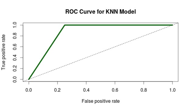
The results are consistent for both the train and test dataset. We are now going to create the ROC curve. This will provide a visual and the AUC number to further help us to assess our model. However, a model is only good when it is compared to another model. Therefore, we will create a really bad model in order to compare it to the original model, and the cross validated model. We will first make a bad model and store the probabilities in the “test” dataset. The bad model will use “age” to predict “Sex” which doesn’t make any sense at all. Below is the code followed by the ROC curve of the bad model.
The more of a diagonal the line is the worst it is. As we can see the bad model is really bad.
What we just did with the bad model we will now repeat for the full model and the cross-validated model. As before, we need to store the prediction in a way that the ROCR package can use them. We will create a variable called “pred.full” to begin the process of graphing the original full model from the last blog post. Then we will use the “prediction” function. Next, we will create the “perf.full” variable to store the performance of the model. Notice, the arguments ‘tpr’ and ‘fpr’ for true positive rate and false positive rate. Lastly, we plot the results
The higher the AUC the better. As such, the full model with all variables is superior to the cross-validated or bad model. This is despite the fact that there are many high correlations in the full model as well. Another point to consider is that the cross-validated model is simpler so this may be a reason to pick it over the full model. As such, the statistics provide support for choosing a model but they do not trump the ability of the research to pick based on factors beyond just numbers.
In this post, we will conduct a logistic regression analysis. Logistic regression is used when you want to predict a categorical dependent variable using continuous or categorical dependent variables. In our example, we want to predict Sex (male or female) when using several continuous variables from the “survey” dataset in the “MASS” package.
data(survey)
?MASS::survey#explains the variables in the study
The first thing we need to do is remove the independent factor variables from our dataset. The reason for this is that the function that we will use for the cross-validation does not accept factors. We will first use the “str” function to identify factor variables and then remove them from the dataset. We also need to remove in examples that are missing data so we use the “na.omit” function for this. Below is the code
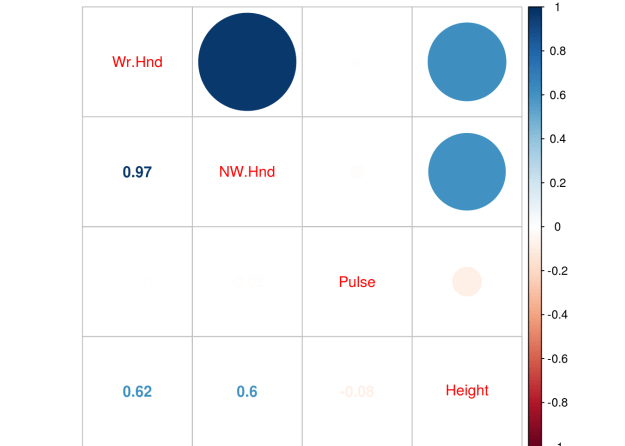
We have an extreme correlation between “We.Hnd” and “NW.Hnd” this makes sense because people’s hands are normally the same size. Since this blog post is a demonstration of logistic regression we will not worry about this too much.
We now need to divide our dataset into a train and a test set. We set the seed for. First, we need to make a variable that we call “ind” that is randomly assigned 70% of the number of rows of survey 1 and 30% 2. We then subset the “train” dataset by taking all rows that are 1’s based on the “ind” variable and we create the “test” dataset for all the rows that line up with 2 in the “ind” variable. This means our data split is 70% train and 30% test. Below is the code
We now make our model. We use the “glm” function for logistic regression. We set the family argument to “binomial”. Next, we look at the results as well as the odds ratios.
fit<-glm(Sex~.,family=binomial,train)summary(fit)
##
## Call:
## glm(formula = Sex ~ ., family = binomial, data = train)
##
## Deviance Residuals:
##     Min       1Q   Median       3Q      Max
## -1.9875  -0.5466  -0.1395   0.3834   3.4443
##
## Coefficients:
##              Estimate Std. Error z value Pr(>|z|)
## (Intercept) -46.42175    8.74961  -5.306 1.12e-07 ***
## Wr.Hnd       -0.43499    0.66357  -0.656    0.512
## NW.Hnd        1.05633    0.70034   1.508    0.131
## Pulse        -0.02406    0.02356  -1.021    0.307
## Height        0.21062    0.05208   4.044 5.26e-05 ***
## Age           0.00894    0.05368   0.167    0.868
## ---
## Signif. codes:  0 '***' 0.001 '**' 0.01 '*' 0.05 '.' 0.1 ' ' 1
##
## (Dispersion parameter for binomial family taken to be 1)
##
##     Null deviance: 169.14  on 122  degrees of freedom
## Residual deviance:  81.15  on 117  degrees of freedom
## AIC: 93.15
##
## Number of Fisher Scoring iterations: 6
The results indicate that only height is useful in predicting if someone is a male or female. The second piece of code shares the odds ratios. The odds ratio tell how a one unit increase in the independent variable leads to an increase in the odds of being male in our model. For example, for every one unit increase in height there is a 1.23 increase in the odds of a particular example being male.
We now need to see how well our model does on the train and test dataset. We first capture the probabilities and save them to the train dataset as “probs”. Next we create a “predict” variable and place the string “Female” in the same number of rows as are in the “train” dataset. Then we rewrite the “predict” variable by changing any example that has a probability above 0.5 as “Male”. Then we make a table of our results to see the number correct, false positives/negatives. Lastly, we calculate the accuracy rate. Below is the code.
Despite the weaknesses of the model with so many insignificant variables it is surprisingly accurate at 88.6%. Let’s see how well we do on the “test” dataset.
As you can see, we do even better on the test set with an accuracy of 93.4%. Our model is looking pretty good and height is an excellent predictor of sex which makes complete sense. However, in the next post we will use cross-validation and the ROC plot to further assess the quality of it.
In this post, we will take a look at best subset regression. Best subset regression fits a model for all possible feature or variable combinations and the decision for the most appropriate model is made by the analyst based on judgment or some statistical criteria.
Best subset regression is an alternative to both Forward and Backward stepwise regression. Forward stepwise selection adds one variable at a time based on the lowest residual sum of squares until no more variables continue to lower the residual sum of squares. Backward stepwise regression starts with all variables in the model and removes variables one at a time. The concern with stepwise methods is they can produce biased regression coefficients, conflicting models, and inaccurate confidence intervals.
Best subset regression bypasses these weaknesses of stepwise models by creating all models possible and then allowing you to assess which variables should be included in your final model. The one drawback to best subset is that a large number of variables means a large number of potential models, which can make it difficult to make a decision among several choices.
In this post, we will use the “Fair” dataset from the “Ecdat” package to predict marital satisfaction based on age, Sex, the presence of children, years married, religiosity, education, occupation, and the number of affairs in the past year. Below is some initial code.
The initial results are already interesting even though the r-square is low. When couples have children the have less marital satisfaction than couples without children when controlling for the other factors and this is the strongest regression weight. In addition, the more education a person has there is an increase in marital satisfaction. Lastly, as the number of affairs increases there is also a decrease in marital satisfaction. Keep in mind that the “rate” variable goes from 1 to 5 with one meaning a terrible marriage to five being a great one. The mean marital satisfaction was 3.52 when controlling for the other variables.
We will now create our subset models. Below is the code.
In the code above we create the sub models using the “regsubsets” function from the “leaps” package and saved it in the variable called “sub.fit”. We then saved the summary of “sub.fit” in the variable “best.summary”. We will use the “best.summary” “sub.fit variables several times to determine which model to use.
There are many different ways to assess the model. We will use the following statistical methods that come with the results from the “regsubset” function.
Mallow’ Cp
Bayesian Information Criteria
We will make two charts for each of the criteria above. The plot to the left will explain how many features to include in the model. The plot to the right will tell you which variables to include. It is important to note that for both of these methods, the lower the score the better the model. Below is the code for Mallow’s Cp.
The plot on the left suggests that a four feature model is the most appropriate. However, this chart does not tell me which four features. The chart on the right is read in reverse order. The high numbers are at the bottom and the low numbers are at the top when looking at the y-axis. Knowing this, we can conclude that the most appropriate variables to include in the model are age, children presence, education, and number of affairs. Below are the results using the Bayesian Information Criterion
These results indicate that a three feature model is appropriate. The variables or features are years married, education, and number of affairs. Presence of children was not considered beneficial. Since our original model and Mallow’s Cp indicated that presence of children was significant we will include it for now.
Below is the code for the model based on the subset regression.
##
## Call:
## lm(formula = rate ~ age + child + education + nbaffairs, data = Fair)
##
## Residuals:
##     Min      1Q  Median      3Q     Max
## -3.2172 -0.7256  0.1675  0.7856  2.2713
##
## Coefficients:
##              Estimate Std. Error t value Pr(>|t|)
## (Intercept)  3.861154   0.307280  12.566  < 2e-16 ***
## age         -0.017440   0.005057  -3.449 0.000603 ***
## childyes    -0.261398   0.103155  -2.534 0.011531 *
## education    0.058637   0.017697   3.313 0.000978 ***
## nbaffairs   -0.084973   0.012830  -6.623 7.87e-11 ***
## ---
## Signif. codes:  0 '***' 0.001 '**' 0.01 '*' 0.05 '.' 0.1 ' ' 1
##
## Residual standard error: 1.029 on 596 degrees of freedom
## Multiple R-squared:  0.1352, Adjusted R-squared:  0.1294
## F-statistic: 23.29 on 4 and 596 DF,  p-value: < 2.2e-16
The results look ok. The older a person is the less satisfied they are with their marriage. If children are present the marriage is less satisfying. The more educated the more satisfied they are. Lastly, the higher the number of affairs indicate less marital satisfaction. However, before we get excited we need to check for collinearity and homoscedasticity. Below is the code
vif(fit2)
##       age     child education nbaffairs
##  1.249430  1.228733  1.023722  1.014338
No issues with collinearity.For vif values above 5 or 10 indicate a problem. Let’s check for homoscedasticity
par(mfrow=c(2,2))plot(fit2)
The normal qqplot and residuals vs leverage plot can be used for locating outliers. The residual vs fitted and the scale-location plot do not look good as there appears to be a pattern in the dispersion which indicates homoscedasticity. To confirm this we will use Breusch-Pagan test from the “lmtest” package. Below is the code
bptest(fit2)
##
##  studentized Breusch-Pagan test
##
## data:  fit2
## BP = 16.238, df = 4, p-value = 0.002716
There you have it. Our model violates the assumption of homoscedasticity. However, this model was developed for demonstration purpose to provide an example of subset regression.
Collecting and preparing data for analysis is the primary job of a data scientist. This experience is called data wrangling. In this post, we will look at an example of data wrangling using a simple artificial data set. You can create the table below in r or excel. If you created it in excel just save it as a csv and load it into r. Below is the initial code
## # A tibble: 10 × 2
##        weight      location
##
## 1         3.2        Europe
## 2       4.2kg       europee
## 3      1.3 kg          U.S.
## 4  7200 grams           USA
## 5          42 United States
## 6         2.3       europee
## 7       2.1kg        Europe
## 8       3.1kg           USA
## 9  2700 grams          U.S.
## 10         24 United States
This a small dataset with the columns of “weight” and “location”. Here are some of the problems
Weights are in different units
Weights are written in different ways
Location is not consistent
In order to have any success with data wrangling, you need to state specifically what it is you want to do. Here are our goals for this project
Convert the “Weight variable” to a numerical variable instead of character
Remove the text and have only numbers in the “weight variable”
Change weights in grams to kilograms
Convert the “location” variable to a factor variable instead of character
Have consistent spelling for Europe and United States in the “location” variable
We will begin with the “weight” variable. We want to convert it to a numerical variable and remove any non-numerical text. Below is the code for this
We use the function “as.numeric” this makes whatever results inside it to be a numerical variable
Inside “as.numeric” we used the “gsub” function which allows us to substitute one value for another.
Inside “gsub” we used the argument pattern and set it to “[[alpha:]]” and “” this told r to look for any lower or uppercase letters and replace with nothing or remove it. This all pertains to the “weight” variable in the apple dataframe.
We now need to convert the weights into grams to kilograms so that everything is the same unit. Below is the code
We used the grep function to search are the “weight” variable in the apple data frame for input that is a digit and is 4 digits in length this is what the “[[:digit:]]{4}” argument means. We do not change any values yet we just store them in “gram.error”
Once this information is stored in “gram.error” we use it as a subset for the “corrected.weight” variable.
We tell r to save into the “corrected.weight” variable any value that is changeable according to the criteria set in “gram.error” and to divide it by 1000. Dividing it by 1000 converts the value from grams to kilograms.
We have completed the transformation of the “weight” and will move to dealing with the problems with the “location” variable in the “apple” dataframe. To do this we will first deal with the issues related to the values that relate to Europe and then we will deal with values related to the United States. Below is the code.
The code is a little complicated to explain but in short We used the “agrep” function to tell r to search the “location” to look for values similar to our term “europe”. The other arguments provide some exceptions that r should change because the exceptions are close to the term europe. This process is repeated for the term “us”. We then store are the location variable from the “apple” dataframe in a new variable called “corrected.location” We then apply the two objects we made called “europe” and “america” to the “corrected.location” variable. Next, we have to make some code to deal with “United States” and apply this using the “gsub” function.
We are almost done, now we combine are two variables “corrected.weight” and “corrected.location” into a new data.frame. The code is below
##    weight location
## 1     3.2   europe
## 2     4.2   europe
## 3     1.3       US
## 4     7.2       US
## 5    42.0       US
## 6     2.3   europe
## 7     2.1   europe
## 8     3.1       US
## 9     2.7       US
## 10   24.0       US
If you use the “str” function on the “cleaned.apple” dataframe you will see that “location” was automatically converted to a factor.
This looks much better especially if you compare it to the original dataframe that is printed at the top of this post.
This post will demonstrate the use of principal component analysis (PCA). PCA is useful for several reasons. One it allows you place your examples into groups similar to linear discriminant analysis but you do not need to know beforehand what the groups are. Second, PCA is used for the purpose of dimension reduction. For example, if you have 50 variables PCA can allow you to reduce this while retaining a certain threshold of variance. If you are working with a large dataset this can greatly reduce the computational time and general complexity of your models.
Keep in mind that there really is not a dependent variable as this is unsupervised learning. What you are trying to see is how different examples can
be mapped in space based on whatever independent variables are used. For our example, we will use the “Carseats” dataset from the “ISLR”. Our goal is to understand the relationship among the variables when examining the shelve location of the car seat. Below is the initial code to begin the analysis
library(ggplot2)library(ISLR)data("Carseats")
We first need to rearrange the data and remove the variables we are not going to use in the analysis. Below is the code.
Here is what we did 1. We made a copy of the “Carseats” data called “Careseats1” 2. We rearranged the order of the variables so that the factor variables are at the end. This will make sense later 3.We removed the “Urban” and “US” variables from the table as they will not be a part of our analysis
We will now do the PCA. We need to scale and center our data otherwise the larger numbers will have a much stronger influence on the results than smaller numbers. Fortunately, the “prcomp” function has a “scale” and a “center” argument. We will also use only the first 7 columns for the analysis as “sheveLoc” is not useful for this analysis. If we hadn’t moved “shelveLoc” to the end of the dataframe it would cause some headache. Below is the code.
The summary of “Carseats.pca” Tells us how much of the variance each component explains. Keep in mind that the number of components is equal to the number of variables. The “proportion of variance” tells us the contribution each component makes and the “cumulative proportion”.
If your goal is dimension reduction than the number of components to keep depends on the threshold you set. For example, if you need around 90% of the variance you would keep the first 5 components. If you need 95% or more of the variance you would keep the first six. To actually use the components you would take the “Carseats.pca$x” data and move it to your data frame.
Keep in mind that the actual components have no conceptual meaning but is a numerical representation of a combination of several variables that were reduced using PCA to fewer variables such as going from 7 variables to 5 variables.
This means that PCA is great for reducing variables for prediction purpose but is much harder for explanatory studies unless you can explain what the new components represent.
For our purposes, we will keep 5 components. This means that we have reduced our dimensions from 7 to 5 while still keeping almost 90% of the variance. Graphing our results is tricky because we have 5 dimensions but the human mind can only conceptualize 3 at the best and normally 2. As such we will plot the first two components and label them by shelf location using ggplot2. Below is the code
From the plot, you can see there is little separation when using the first two components of the PCA analysis. This makes sense as we can only graph to components so we are missing a lot of the variance. However, for demonstration purposes the analysis is complete.
In this post we will look at an example of linear discriminant analysis (LDA). LDA is used to develop a statistical model that classifies examples in a dataset. In the example in this post, we will use the “Star” dataset from the “Ecdat” package. What we will do is try to predict the type of class the students learned in (regular, small, regular with aide) using their math scores, reading scores, and the teaching experience of the teacher. Below is the initial code
library(Ecdat)
library(MASS)
data(Star)
We first need to examine the data by using the “str” function
The data mostly looks good. The results of the “prop.table” function will help us when we develop are training and testing datasets. The only problem is with the “totexpk” variable. IT is not anywhere near to be normally distributed. TO deal with this we will use the square root for teaching experience. Below is the code
None of the correlations are too bad. We can now develop our model using linear discriminant analysis. First, we need to scale are scores because the test scores and the teaching experience are measured differently. Then, we need to divide our data into a train and test set as this will allow us to determine the accuracy of the model. Below is the code.
Now we develop our model. In the code before the “prior” argument indicates what we expect the probabilities to be. In our data the distribution of the the three class types is about the same which means that the apriori probability is 1/3 for each class type.
The printout is mostly readable. At the top is the actual code used to develop the model followed by the probabilities of each group. The next section shares the means of the groups. The coefficients of linear discriminants are the values used to classify each example. The coefficients are similar to regression coefficients. The computer places each example in both equations and probabilities are calculated. Whichever class has the highest probability is the winner. In addition, the higher the coefficient the more weight it has. For example, “tmathssk” is the most influential on LD1 with a coefficient of 0.89.
The proportion of trace is similar to principal component analysis
Now we will take the trained model and see how it does with the test set. We create a new model called “predict.lda” and use are “train.lda” model and the test data called “test.star”
predict.lda<-predict(train.lda,newdata=test.star)
We can use the “table” function to see how well are model has done. We can do this because we actually know what class our data is beforehand because we divided the dataset. What we need to do is compare this to what our model predicted. Therefore, we compare the “classk” variable of our “test.star” dataset with the “class” predicted by the “predict.lda” model.
The results are pretty bad. For example, in the first row called “regular” we have 155 examples that were classified as “regular” and predicted as “regular” by the model. In rhe next column, 182 examples that were classified as “regular” but predicted as “small.class”, etc. To find out how well are model did you add together the examples across the diagonal from left to right and divide by the total number of examples. Below is the code
(155+198+269)/1748
## [1] 0.3558352
Only 36% accurate, terrible but ok for a demonstration of linear discriminant analysis. Since we only have two-functions or two-dimensions we can plot our model. Below I provide a visual of the first 50 examples classified by the predict.lda model.
The first function, which is the vertical line, doesn’t seem to discriminant anything as it off to the side and not separating any of the data. However, the second function, which is the horizontal one, does a good of dividing the “regular.with.aide” from the “small.class”. Yet, there are problems with distinguishing the class “regular” from either of the other two groups. In order improve our model we need additional independent variables to help to distinguish the groups in the dependent variable.
In this post, we will learn how to create a generalized additive model (GAM). GAMs are non-parametric generalized linear models. This means that linear predictor of the model uses smooth functions on the predictor variables. As such, you do not need to specify the functional relationship between the response and continuous variables. This allows you to explore the data for potential relationships that can be more rigorously tested with other statistical models
In our example, we will use the “Auto” dataset from the “ISLR” package and use the variables “mpg”,“displacement”,“horsepower”, and “weight” to predict “acceleration”. We will also use the “mgcv” package. Below is some initial code to begin the analysis
library(mgcv)
library(ISLR)data(Auto)
We will now make the model we want to understand the response of “acceleration” to the explanatory variables of “mpg”,“displacement”,“horsepower”, and “weight”. After setting the model we will examine the summary. Below is the code
All of the explanatory variables are significant and the adjust r-squared is .73 which is excellent. edf stands for “effective degrees of freedom”. This modified version of the degree of freedoms is due to the smoothing process in the model. GCV stands for generalized cross-validation and this number is useful when comparing models. The model with the lowest number is the better model.
We can also examine the model visually by using the “plot” function. This will allow us to examine if the curvature fitted by the smoothing process was useful or not for each variable. Below is the code.
plot(model1)
We can also look at a 3d graph that includes the linear predictor as well as the two strongest predictors. This is done with the “vis.gam” function. Below is the code
vis.gam(model1)
If multiple models are developed. You can compare the GCV values to determine which model is the best. In addition, another way to compare models is with the “AIC” function. In the code below, we will create an additional model that includes “year” compare the GCV scores and calculate the AIC. Below is the code.
As you can see, the second model has a higher GCV score when compared to the first model. This indicates that the first model is a better choice. This makes sense because in the second model the variable “year” is not significant. To confirm this we will calculate the AIC scores using the AIC function.
Again, you can see that model1 s better due to its fewer degrees of freedom and slightly lower AIC score.
Conclusion
Using GAMs is most common for exploring potential relationships in your data. This is stated because they are difficult to interpret and to try and summarize. Therefore, it is normally better to develop a generalized linear model over a GAM due to the difficulty in understanding what the data is trying to tell you when using GAMs.
Generalized linear models are another way to approach linear regression. The advantage of of GLM is that allows the error to follow many different distributions rather than only the normal distribution which is an assumption of traditional linear regression.
Often GLM is used for response or dependent variables that are binary or represent count data. THis post will provide a brief explanation of GLM as well as provide an example.
Key Information
There are three important components to a GLM and they are
Error structure
Linear predictor
Link function
The error structure is the type of distribution you will use in generating the model. There are many different distributions in statistical modeling such as binomial, gaussian, poission, etc. Each distribution comes with certain assumptions that govern their use.
The linear predictor is the sum of the effects of the independent variables. Lastly, the link function determines the relationship between the linear predictor and the mean of the dependent variable. There are many different link functions and the best link function is the one that reduces the residual deviances the most.
In our example, we will try to predict if a house will have air conditioning based on the interactioon between number of bedrooms and bathrooms, number of stories, and the price of the house. To do this, we will use the “Housing” dataset from the “Ecdat” package. Below is some initial code to get started.
library(Ecdat)
data("Housing")
The dependent variable “airco” in the “Housing” dataset is binary. This calls for us to use a GLM. To do this we will use the “glm” function in R. Furthermore, in our example, we want to determine if there is an interaction between number of bedrooms and bathrooms. Interaction means that the two independent variables (bathrooms and bedrooms) influence on the dependent variable (aircon) is not additive, which means that the combined effect of the independnet variables is different than if you just added them together. Below is the code for the model followed by a summary of the results
##
## Call:
## glm(formula = Housing$airco ~ Housing$bedrooms * Housing$bathrms +
##     Housing$stories + Housing$price, family = binomial)
##
## Deviance Residuals:
##     Min       1Q   Median       3Q      Max
## -2.7069  -0.7540  -0.5321   0.8073   2.4217
##
## Coefficients:
##                                    Estimate Std. Error z value Pr(>|z|)
## (Intercept)                      -6.441e+00  1.391e+00  -4.632 3.63e-06
## Housing$bedrooms                  8.041e-01  4.353e-01   1.847   0.0647
## Housing$bathrms                   1.753e+00  1.040e+00   1.685   0.0919
## Housing$stories                   3.209e-01  1.344e-01   2.388   0.0170
## Housing$price                     4.268e-05  5.567e-06   7.667 1.76e-14
## Housing$bedrooms:Housing$bathrms -6.585e-01  3.031e-01  -2.173   0.0298
##
## ---
## Signif. codes:  0 '***' 0.001 '**' 0.01 '*' 0.05 '.' 0.1 ' ' 1
##
## (Dispersion parameter for binomial family taken to be 1)
##
##     Null deviance: 681.92  on 545  degrees of freedom
## Residual deviance: 549.75  on 540  degrees of freedom
## AIC: 561.75
##
## Number of Fisher Scoring iterations: 4
To check how good are model is we need to check for overdispersion as well as compared this model to other potential models. Overdispersion is a measure to determine if there is too much variablity in the model. It is calcualted by dividing the residual deviance by the degrees of freedom. Below is the solution for this
549.75/540
## [1] 1.018056
Our answer is 1.01, which is pretty good because the cutoff point is 1, so we are really close.
Now we will make several models and we will compare the results of them
Model 2
#add recroom and garageplmodel2<-glm(Housing$airco~Housing$bedrooms*Housing$bathrms+Housing$stories+Housing$price+Housing$recroom+Housing$garagepl, family=binomial)summary(model2)
##
## Call:
## glm(formula = Housing$airco ~ Housing$bedrooms * Housing$bathrms +
##     Housing$stories + Housing$price + Housing$recroom + Housing$garagepl,
##     family = binomial)
##
## Deviance Residuals:
##     Min       1Q   Median       3Q      Max
## -2.6733  -0.7522  -0.5287   0.8035   2.4239
##
## Coefficients:
##                                    Estimate Std. Error z value Pr(>|z|)
## (Intercept)                      -6.369e+00  1.401e+00  -4.545 5.51e-06
## Housing$bedrooms                  7.830e-01  4.391e-01   1.783   0.0745
## Housing$bathrms                   1.702e+00  1.047e+00   1.626   0.1039
## Housing$stories                   3.286e-01  1.378e-01   2.384   0.0171
## Housing$price                     4.204e-05  6.015e-06   6.989 2.77e-12
## Housing$recroomyes                1.229e-01  2.683e-01   0.458   0.6470
## Housing$garagepl                  2.555e-03  1.308e-01   0.020   0.9844
## Housing$bedrooms:Housing$bathrms -6.430e-01  3.054e-01  -2.106   0.0352
##
## ---
## Signif. codes:  0 '***' 0.001 '**' 0.01 '*' 0.05 '.' 0.1 ' ' 1
##
## (Dispersion parameter for binomial family taken to be 1)
##
##     Null deviance: 681.92  on 545  degrees of freedom
## Residual deviance: 549.54  on 538  degrees of freedom
## AIC: 565.54
##
## Number of Fisher Scoring iterations: 4
The results of the anova indicate that the models are all essentially the same as there is no statistical difference. The only criteria on which to select a model is the measure of overdispersion. The first model has the lowest rate of overdispersion and so is the best when using this criteria. Therefore, determining if a hous has air conditioning depends on examining number of bedrooms and bathrooms simultenously as well as the number of stories and the price of the house.
Conclusion
The post explained how to use and interpret GLM in R. GLM can be used primarilyy for fitting data to disrtibutions that are not normal.
Proportions are a fraction or “portion” of a total amount. For example, if there are ten men and ten women in a room the proportion of men in the room is 50% (5 / 10). There are times when doing an analysis that you want to evaluate proportions in our data rather than individual measurements of mean, correlation, standard deviation etc.
In this post we will learn how to do a test of proportions using R. We will use the dataset “Default” which is found in the “ISLR” package. We will compare the proportion of those who are students in the dataset to a theoretical value. We will calculate the results using the z-test and the binomial exact test. Below is some initial code to get started.
library(ISLR)data("Default")
We first need to determine the actual number of students that are in the sample. This is calculated below using the “table” function.
table(Default$student)
##
## No Yes
## 7056 2944
We have 2944 students in the sample and 7056 people who are not students. We now need to determine how many people are in the sample. If we sum the results from the table below is the code.
sum(table(Default$student))
## [1] 10000
There are 10000 people in the sample. To determine the proportion of students we take the number 2944 / 10000 which equals 29.44 or 29.44%. Below is the code to calculate this
The proportion test compares a particular value with a theoretical value. For our example, the particular value we have is 29.44% of the people were students. We want to compare this value with a theoretical value of 50%. Before we do so it is better to state specificallt what are hypotheses are. NULL = The value of 29.44% of the sample being students is the same as 50% found in the population ALTERNATIVE = The value of 29.44% of the sample being students is NOT the same as 50% found in the population.
##
## 1-sample proportions test without continuity correction
##
## data: 2944 out of 10000, null probability 0.5
## X-squared = 1690.9, df = 1, p-value < 2.2e-16
## alternative hypothesis: true p is not equal to 0.5
## 95 percent confidence interval:
## 0.2855473 0.3034106
## sample estimates:
## p
## 0.2944
Here is what the code means. 1. prop.test is the function used 2. The first value of 2944 is the total number of students in the sample 3. n = is the sample size 4. p= 0.5 is the theoretical proportion 5. alternative =“two.sided” means we want a two-tail test 6. correct = FALSE means we do not want a correction applied to the z-test. This is useful for small sample sizes but not for our sample of 10000
The p-value is essentially zero. This means that we reject the null hypothesis and conclude that the proportion of students in our sample is different from a theortical proportion of 50% in the population.
Below is the same analysis using the binomial exact test.
binom.test(2944, n=10000, p=0.5)
##
## Exact binomial test
##
## data: 2944 and 10000
## number of successes = 2944, number of trials = 10000, p-value <
## 2.2e-16
## alternative hypothesis: true probability of success is not equal to 0.5
## 95 percent confidence interval:
## 0.2854779 0.3034419
## sample estimates:
## probability of success
## 0.2944
The results are the same. Whether to use the “prop.test”” or “binom.test” is a major argument among statisticians. The purpose here was to provide an example of the use of both
This post will explore an example of testing if a dataset fits a specific theoretical distribution. This is a very important aspect of statistical modeling as it allows to understand the normality of the data and the appropriate steps needed to take to prepare for analysis.
In our example, we will use the “Auto” dataset from the “ISLR” package. We will check if the horsepower of the cars in the dataset is normally distributed or not. Below is some initial code to begin the process.
library(ISLR)library(nortest)library(fBasics)
data("Auto")
Determining if a dataset is normally distributed is simple in R. This is normally done visually through making a Quantile-Quantile plot (Q-Q plot). It involves using two functions the “qnorm” and the “qqline”. Below is the code for the Q-Q plot
qqnorm(Auto$horsepower)
We now need to add the Q-Q line to see how are distribution lines up with the theoretical normal one. Below is the code. Note that we have to repeat the code above in order to get the completed plot.
The “qqline” function needs the data you want to test as well as the distribution and probability. The distribution we wanted is normal and is indicated by the argument “qnorm”. The probs argument means probability. The default values are .25 and .75. The resulting graph indicates that the distribution of “horsepower”, in the “Auto” dataset is not normally distributed. That are particular problems with the lower and upper values.
We can confirm our suspicion by running a statistical test. The Anderson-Darling test from the “nortest” package will allow us to test whether our data is normally distributed or not. The code is below
ad.test(Auto$horsepower)
## Anderson-Darling normality test
##
## data: Auto$horsepower
## A = 12.675, p-value < 2.2e-16
From the results, we can conclude that the data is not normally distributed. This could mean that we may need to use non-parametric tools for statistical analysis.
We can further explore our distribution in terms of its skew and kurtosis. Skew measures how far to the left or right the data leans and kurtosis measures how peaked or flat the data is. This is done with the “fBasics” package and the functions “skewness” and “kurtosis”.
First we will deal with skewness. Below is the code for calculating skewness.
We now need to determine if this value of skewness is significantly different from zero. This is done with a simple t-test. We must calculate the t-value before calculating the probability. The standard error of the skew is defined as the square root of six divided by the total number of samples. The code is below
Now we take the standard error of Horsepower and plug this into the “pt” function (t probability) with the degrees of freedom (sample size – 1 = 391) we also put in the number 1 and subtract all of this information. Below is the code
1-pt(stdErrorHorsepower,391)
## [1] 0
## attr(,"method")
## [1] "moment"
The value zero means that we reject the null hypothesis that the skew is not significantly different form zero and conclude that the skew is different form zero. However, the value of the skew was only 1.1 which is not that non-normal.
We will now repeat this process for the kurtosis. The only difference is that instead of taking the square root divided by six we divided by 24 in the example below.
Again the pvalue is essentially zero, which means that the kurtosis is significantly different from zero. With a value of 2.64 this is not that bad. However, when both skew and kurtosis are non-normally it explains why our overall distributions was not normal either.
Conclusion
This post provided insights into assessing the normality of a dataset. Visually inspection can take place using Q-Q plots. Statistical inspection can be done through hypothesis testing along with checking skew and kurtosis.
In this post, we will use probability distributions and ggplot2 in R to solve a hypothetical example. This provides a practical example of the use of R in everyday life through the integration of several statistical and coding skills. Below is the scenario.
At a busing company the average number of stops for a bus is 81 with a standard deviation of 7.9. The data is normally distributed. Knowing this complete the following.
Calculate the interval value to use using the 68-95-99.7 rule
Calculate the density curve
Graph the normal curve
Evaluate the probability of a bus having less then 65 stops
Evaluate the probability of a bus having more than 93 stops
Calculate the Interval Value
Our first step is to calculate the interval value. This is the range in which 99.7% of the values falls within. Doing this requires knowing the mean and the standard deviation and subtracting/adding the standard deviation as it is multiplied by three from the mean. Below is the code for this.
The values above mean that we can set are interval between 55 and 110 with 100 buses in the data. Below is the code to set the interval.
interval<-seq(55,110, length=100)#length here represents
100 fictitious buses
Density Curve
The next step is to calculate the density curve. This is done with our knowledge of the interval, mean, and standard deviation. We also need to use the “dnorm” function. Below is the code for this.
densityCurve<-dnorm(interval,mean=81,sd=7.9)
We will now plot the normal curve of our data using ggplot. Before we need to put our “interval” and “densityCurve” variables in a dataframe. We will call the dataframe “normal” and then we will create the plot. Below is the code.
library(ggplot2)normal<-data.frame(interval, densityCurve)ggplot(normal, aes(interval, densityCurve))+geom_line()+ggtitle("Number of Stops for Buses")
Probability Calculation
We now want to determine what is the provability of a bus having less than 65 stops. To do this we use the “pnorm” function in R and include the value 65, along with the mean, standard deviation, and tell R we want the lower tail only. Below is the code for completing this.
pnorm(65,mean=81,sd=7.9,lower.tail=TRUE)
## [1] 0.02141744
As you can see, at 2% it would be unusually to. We can also plot this using ggplot. First, we need to set a different density curve using the “pnorm” function. Combine this with our “interval” variable in a dataframe and then use this information to make a plot in ggplot2. Below is the code.
CumulativeProb<-pnorm(interval, mean=81,sd=7.9,lower.tail=TRUE)pnormal<-data.frame(interval, CumulativeProb)ggplot(pnormal, aes(interval, CumulativeProb))+geom_line()+ggtitle("Cumulative Density of Stops for Buses")
Second Probability Problem
We will now calculate the probability of a bus have 93 or more stops. To make it more interesting we will create a plot that shades the area under the curve for 93 or more stops. The code is a little to complex to explain so just enjoy the visual.
pnorm(93,mean=81,sd=7.9,lower.tail=FALSE)
## [1] 0.06438284
x<-intervalytop<-dnorm(93,81,7.9)MyDF<-data.frame(x=x,y=densityCurve)p<-ggplot(MyDF,aes(x,y))+geom_line()+scale_x_continuous(limits=c(50, 110))
+ggtitle("Probabilty of 93 Stops or More is 6.4%")shade<-rbind(c(93,0), subset(MyDF, x>93), c(MyDF[nrow(MyDF), "X"], 0))p+geom_segment(aes(x=93,y=0,xend=93,yend=ytop))+geom_polygon(data=shade, aes(x, y))
Conclusion
A lot of work was done but all in a practical manner. Looking at realistic problem. We were able to calculate several different probabilities and graph them accordingly.
It seems as though there are no limits to what can be done with ggplot2. Another example of this is the use of maps in presenting data. If you are trying to share information that depends on location then this is an important feature to understand.
This post will provide some basic explanation for understanding how to use maps with ggplot2.
The Maps Package
One of several packages available for using maps with ggplot2 is the “maps” package. This package contains a limited number of maps along with several databases that contain information that can be used to create data-filled maps.
The “maps” package cooperates with ggplot2 through the use of the “borders” function and plotting the plot using lattitude and longitude for the “aes” function. After you have installed the “maps” package you can run the example code below.
In the code above we told R to use the data from “us.cities” which comes with the “maps” package. We then told R to graph the latitude and longitude and to do this by placing a point for each city. Lastly, the “borders” function was use to place this information on the state map of the US.
There are several points way off of the map. These represents datapoints for cities in Alaska and Hawaii.
Below is an example that is limited to one state in America. To do this we first must subset the data to only include one state.
In the example above, we took all of the cities in Thailand and saved them into the variable “Thai_cities”. We then made a plot of Thailand but we played with the color and fill features. Lastly, we plotted the population be location and we indicated that the size of the data point should depend on the size. In this example, all the data points were the same size which means that all the cities in Thailand in the dataset are about the same size.
We can also add text to maps. In the example below, we will use a subset of the data from Thailand and add the names of cities to the map.
In this plot there is a messy part in the middle where Bangkok is a long with several other large cities. However, you can see the flexiability in the plot by adding the “geom_text” function which has been discussed previously. In the “geom_text” function we added some aesthetics as well add the “name” of the city.
Conclusion
In this post, we look at some of the basic was of using maps with ggplot2. There are many more ways and features that can be explored in future post.
This post will provide explanation on how to customize the axis and title of a plot that utilizes ggplot2. We will use the “Computer” dataset from the “Ecdat” package looking specifically at the difference in price of computers based on the inclusion of a cd-rom. Below is some code needed to be prepared for the examples along with a printout of our initial boxplot.
In the example below, we change the color of the tick marks to purple and we bold them. This all involves the use of the “axis.text” argument in the “theme” function.
In the example below, the y label “price” is rotated 90 degrees to be in line with text. This is accomplished using the “axis.title.y” argument along with additional code.
It is also possible to modify the plot background axis as well. In the example below, we change the background color to blue, the color of the lines to green, and yellow.
This is not an attractive plot but it does provide an example of the various options available in ggplot2
All of the tricks we have discussed so far can also apply when faceting data. Below we make a scatterplot using the same background as before but comparing trend and price.
Right now the plots are too close to each other. We can account for this by modifying the panel margins.
theScatter1+theme(panel.margin=unit(2,"cm"))
Conclusion
These examples provide further evidence of the endless variety that is available when using ggplot2. Whatever are your purposes, it is highly probably that ggplot2 has some sort of a data visualization answer.
This post will provide information on fine tuning the legend of a graph using ggplot2. We will be using the “Wage” dataset from the “ISLR” package. Below is some initial code that is needed to complete the examples. The initial plot is saved as a variable to save time and avoid repeating the same code.
The default ggplot has a grey background with grey text. By adding the “theme_bw” function to a plot you can create a plot that has a white background with black text. The code is below.
myBoxplot+theme_bw()
If you desire, you can also add a rectangle around the legend with the “legend.baclground” argument You can even specify the color of the rectangle as shown below.
It is also possible to add a highlighting color to the keys in the legend. In the code below we highlight the keys with the color red using the “legend.key” argument
The code below provides an example of how to change the size of a plot.
myBoxplot+theme(legend.margin=unit(2, "cm"))
This example demonstrate how to modify the text in a legend. This requires the use of the “legend.text”, along with several other arguments and functions. The code below does the following.
Lastly, you can even move the legend around the plot. The first example moves the legend to the top of the plot using “legend.position” argument. The second example moves the legend based on numerical input. The first number moves the plot from left to right or from 0 being left to 1 being all the way to the right. The second number moves the text from bottom to top with 0 being the bottom and 1 being the top.
myBoxplot+theme(legend.position="top")
myBoxplot+theme(legend.position=c(.6,.7))
Conclusion
The examples provided here show how much control over plots is possible when using ggplot2. In many ways this is just an introduction into the nuance controlled that is available
In this post, we will look at how to manipulate the labels and positioning of the data when using ggplot2. We will use the “Wage” data from the “ISLR” package. Below is initial code needed to begin.
library(ggplot2);library(ISLR)data("Wage")
Manipulating Labels
Our first example involves adding labels for the x, y-axis as well as a title. To do this we will create a histogram of the wage variable and save it as a variable in R. By saving the histogram as a variable it saves time as we do not have to recreate all of the code but only add the additional information. After creating the histogram and saving it to a variable we will add the code for creating the labels. Below is the code
myHistogram<-ggplot(Wage, aes(wage, fill=..count..))+geom_histogram()myHistogram+labs(title="This is My Histogram", x="Salary as a Wage", y="Number")
By using the “labs” function you can add a title and information for the x and y-axis. If your title is really long you can use the code “” to break the information into separate lines as shown below.
myHistogram+labs(title="This is the Longest Title for a Histogram \n that I have ever Seen in My Entire Life", x="Salary as a Wage", y="Number")
Discrete Axis Scale
We will now turn our attention to working with discrete scales. Discrete scales deal with categorical data such as box plots and bar charts. First, we will store a boxplot of the wages subsetted by the level of education in a variable and we will display it.
Now, by using the “scale_x_discrete” function along with the “limits” argument we are able to change the order of the groups as shown below
myBoxplot+scale_x_discrete(limits=c("5. Advanced Degree","2. HS Grad","1. < HS Grad","4. College Grad","3. Some College"))
Continuous Scale
The most common modification to a continuous scale is to modify the range. In the code below, we change the default range of “myBoxplot” to something that is larger.
myBoxplot+scale_y_continuous(limits=c(0,400))
Conclusion
This post provided some basic insights into modifying plots using ggplot2.
This post will explain several types of visuals that can be developed in using ggplot2. In particular, we are going to make three specific types of charts and they are…
Pie chart
Bullseye chart
Coxcomb diagram
To complete this task, we will use the “Wage” dataset from the “ISLR” package. We will use the “education” variable which has five factors in it. Below is the initial code to get started.
library(ggplot2);library(ISLR)data("Wage")
Pie Chart
In order to make a pie chart, we first need to make a bar chart and add several pieces of code to change it into a pie chart. Below is the code for making a regular bar plot.
We will now modify two parts of the code. First, we do not want separate bars. Instead, we want one bar. The reason being is that we only want one pie chart so before that we need one bar. Therefore, for the x value in the “aes” function, we will use the argument “factor(1)” which tells R to force the data as one factor on the chart thus making one bar. We also need to add the “width=1” inside the “geom_bar” function. This helps with spacing. Below is the code for this
To make the pie chart, we need to add the “coord_polar” function to the code which adjusts the mapping. We will include the argument “theta=y” which tells R that the size of the pie a factor gets depends on the number of people in that factor. Below is the code for the pie chart.
A bullseye chart is a pie chart that shares the information in a concentric way. The coding is mostly the same except that you remove the “theta” argument from the “coord_polar” function. The thicker the circle the more respondents within it. Below is the code
The Coxcomb Diagram is similar to the pie chart but the data is not normalized to fit the entire area of the circle. To make this plot we have to modify the code to make the by removing the “factor(1)” argument and replacing it with the name of the variable and be reading the “coord_polor” function. Below is the code
These are just some of the many forms of visualizations available using ggplot2. Which to use depends on many factors from personal preference to the needs of the audience.
In this post, we will look at how ggplot2 is able to create variables for the purpose of providing aesthetic information for a histogram. Specifically, we will look at how ggplot2 calculates the bin sizes and then assigns colors to each bin depending on the count or density of that particular bin.
To do this we will use dataset called “Star” from the “Edat” package. From the dataset, we will look at total math score and make several different histograms. Below is the initial code you need to begin.
library(ggplot2);library(Ecdat)
data(Star)
We will now create our initial histogram. What is new in the code below is the “..count..” for the “fill” argument. This information tells are to fill the bins based on their count or the number of data points that fall in this bin. By doing this, we get a gradation of colors with darker colors indicating more data points and lighter colors indicating fewer data points. The code is as follows.
As you can see, we have a nice histogram that uses color to indicate how common data in a specific bin is. We can also make a histogram that has a line that indicates the density of the data using the kernel function. This is similar to adding a LOESS line on a plot. The code is below.
The code is mostly the same but we moved the “fill” argument inside “geom_histogram” function and added a second “aes” function. We also included a y argument inside the second “aes” function. Instead of using the “..count..” information we used “..density..” as this is needed to create the line. Lastly, we added the “geom_density” function.
The chart below uses the “alpha” argument to add transparency to the histogram. This allows us to communicate additional information. In the histogram below we can see visual information about gender and the how common a particular gender and bin are in the data.
What we have learned in this post is some of the basic features of ggplot2 for creating various histograms. Through the use of colors, a researcher is able to display useful information in an interesting way.
In this post, we will look at how to add a regression line to a plot using the “ggplot2” package. This is mostly a review of what we learned in the post on adding a LOESS line to a plot. The main difference is that a regression line is a straight line that represents the relationship between the x and y variable while a LOESS line is used mostly to identify trends in the data.
One new wrinkle we will add to this discussion is the use of faceting when developing plots. Faceting is the development of multiple plots simultaneously with each sharing different information about the data.
The data we will use is the “Housing” dataset from the “Ecdat” package. We will examine how lotsize affects housing price when also considering whether the house has central air conditioning or not. Below is the initial code in order to be prepared for analysis
library(ggplot2);library(Ecdat)
## Loading required package: Ecfun
##
## Attaching package: 'Ecdat'
##
## The following object is masked from 'package:datasets':
##
## Orange
data("Housing")
The first plot we will make is the basic plot of lotsize and price with the data being distinguished by having central air or not, without a regression line. The code is as follows
We will now experiment with a technique called faceting. Faceting allows you to split the data by various subgroups and display the result via plot simultaneously. For example, below is the code for splitting the data by central air for examining the relationship between lot size and price.
By adding the “facet_grid” function we can subset the data by the categorical variable “airco”.
In the code below we have three plots. The first two show the relationship between lotsize and price based on central air and the last plot shows the overall relationship.
By adding the argument “margins” and setting it to true we are able to add the third plot that shows the overall results.
So far all of are facetted plots have had the same statistical transformation of the use of a regression. However, we can actually mix the type of transformations that happen when facetting the results. This is shown below.
In the code we needed to use two functions of “stat_smooth” and indicate the information to transform inside the function. The plot to the left is a regression line with houses without central air and the plot to the right is a LOESS line with houses that have central air.
Conclusion
In this post, we explored the use of regression lines and advance faceting techniques. Communicating data with ggplot2 is one of many ways in which a data analyst can portray valuable information.
A common goal of statistics is to try and identify trends in the data as well as to predict what may happen. Both of these goals can be partially achieved through the development of graphs and or charts.
In this post, we will look at adding a smooth line to a scatterplot using the “ggplot2” package.
To accomplish this, we will use the “Carseats” dataset from the “ISLR” package. We will explore the relationship between the price of carseats with actual sales along with whether the carseat was purchase in an urban location or not. Below is some initial code to prepare for the analysis.
library(ggplot2);library(ISLR)data("Carseats")
We are going to use a layering approach in this example. This means we will add one piece of code at a time until we have the complete plot.We are now going to plot the initial scatterplot. We simply want a scatterplot depicting the relationship between Price and Sales of carseats.
The general trend appears to be negative. As price increases sales decrease regardless if carseat was purchase in an urban setting or not.
We will now add ar LOESS line to the graph. LOESS stands for “Locally weighted smoothing” this is a commonly used tool in regression analysis. The addition of a LOESS line allows in identifying trends visually much easily. Below is the code
Unlike a regression line which is strictly straight, a LOESS line curves with the data. As you look at the graph the LOESS line is mostly straight with curves at the extremes and for a small rise in fall in the middle for carseats purchased in urban areas.
So far we have created LOESS lines by the categorical variable Urban. We can actually make a graph with three LOESS lines. One for Yes urban, another for No Urban, and the last one that is an overall line that does not take into account the Urban variable. Below is the code.
Notice that the code is slightly different with the information being mostly outside of the “ggplot” function. You can barely see the third line in the graph but if you look closely you will see a new blue line that was not there previously. This is the overall trend line. If you want you can see the overall trend line with the code below.
The very first graph we generated in this post only contained points. This is because we used the “geom_point” function. Any of the graphs we created could be generated with points by removing the “geom_point” function and only using the “stat_smooth” function as shown below.
This post provided an introduction to adding LOESS lines to a graph using ggplot2. For presenting data in a visually appealing way, adding lines can help in identifying key characteristics in the data.
In developing graphs, there are certain core principles that need to be addressed in order to provide a graph that communicates meaning clearly to an audience. Many of these core principles are addressed in the book “The Grammar of Graphics” by Leland Wilkinson.
The concepts of Wilkinson’s book were used to create the “ggplot2” r package by Hadley Wickham. This post will explain some of the core principles needed in developing high-quality visualizations. In particular, we will look at the following.
Aesthetic attributes
Geometric objects
Statistical transformations
Scales
Coordinates
Faceting
One important point to mention is that when using ggplot2 not all of these concepts have to be addressed in the code as R will auto-select certain features if you do not specify them.
Aesthetic Attributes and Geometric Objects
Aesthetic attributes are about how the data is perceived. This generally involves arguments in the “ggplot” relating to the x/y coordinates as well as the actual data that is being used. Aesthetic attributes are mandatory information for making a graph.
Geometric objects determine what type of plot is generated. There are many different examples such as bar, point, boxplot, and histogram.
To use the “ggplot” function you must provide the aesthetic and geometric object information to generate a plot. Below is coding containing only this information.
## `stat_bin()` using `bins = 30`. Pick better value with `binwidth`.
The code is broken down as follows ggplot (data, aesthetic attribute(x-axis data at least)+geometric object())
Statistical Transformation Statistical transformation involves combining the data in one way or the other to get a general sense of the data. Examples of statistical transformation include adding a smooth line, a regression line, or even binning the data for histograms. This feature is optional but can provide additional explanation of the data.
Below we are going to look at two variables on one plot. For this, we will need a different geometric object as we will use points instead of a histogram. We will also use a statistical transformation. In particular, the statistical transformation is regression line. The code is as follows
The code is broken down as follows ggplot (data, aesthetic attribute(x-axis data at least)+geometric object()+ statistical transformation(type of transformation))
Scales Scales is a rather complicated feature. For simplicity, scales have to do with labeling the title, x and y-axis, creating a legend, as well as the coloring of data points. This use of this feature is optional.
Below is a simple example using the “labs” function in the plot we develop in the previous example.
ggplot(Orange, aes(circumference,age))+geom_point()+stat_smooth(method="lm")+labs(title="Example Plot", x="circumference of the tree", y="age of the tree")
The plot now has a title and clearly labeled x and y axises
Coordinates Coordinates is another complex feature. This feature allows for the adjusting of the mapping of the data. Two common mapping features are cartesian and polar. Cartesian is commonly used for plots in 2D while polar is often used for pie charts.
In the example below, we will use the same data but this time use a polar mapping approach. The plot doesn’t make much sense but is really just an example of using this feature. This feature is also optional.
ggplot(Orange, aes(circumference, age))+geom_point()+stat_smooth(method="lm")+labs(title="Example Plot",x="circumference of the tree", y="age of the tree")+coord_polar()
The last feature is faceting. Faceting allows you to group data in subsets. This allows you to look at your data from the perspective of various subgroups in the sample population.
In the example below, we will look at the relationship between circumference and age by tree type.
ggplot(Orange, aes(circumference, age))+geom_point()+stat_smooth(method="lm")+labs(title="Example Plot",x="circumference of the tree", y="age of the tree")+facet_grid(Tree~.)
Now we can see the relationship between the two variables based on the type of tree. One important thing to note about the “facet_grid” function is the use of the “.~” If this symbol “~.” is placed behind the categorical variable the charts will be stacked on top of each other is in the previous example.
However, if the symbol is written differently “.~” and placed in front of the categorical variable the plots will be placed next to each other as in the example below
ggplot(Orange, aes(circumference, age))+geom_point()+stat_smooth(method="lm")+labs(title="Example Plot",x="circumference of the tree", y="age of the tree")+facet_grid(.~Tree)
Conclusion
This post provided an introduction to the grammar of graphics. In order to appreciate the art of data visualization, it requires understanding how the different principles of graphics work together to communicate information in a visual manner with an audience.
In this post, we will explore the use of the “qplot” function from the “ggplot2” package. One of the major advantages of “ggplot” when compared to the base graphics package in R is that the “ggplot2” plots are much more visually appealing. This will make more sense when we explore the grammar of graphics. for now, we will just make plots to get used to using the “qplot” function.
We are going to use the “Carseats” dataset from the “ISLR” package in the examples. This dataset has data about the purchase of carseats for babies. Below is the initial code you will need to make the various plots.
library(ggplot2);library(ISLR)data("Carseats")
In the first scatterplot, we are going to compare the price of a carseat with the volume of sales. Below is the code
qplot(Price, Sales,data=Carseats)
Most of this coding format you are familiar. “Price” is the x variable. “Sales” is the y variable and the data used is “Carseats. From the plot, we can see that as the price of the carseat increases there is normally a decline in the number of sales.
For our next plot, we will compare sales based on shelf location. This requires the use of a boxplot. Below is the code
The new argument in the code is the “geom” argument. This argument indicates what type of plot is drawn.
The boxplot appears to indicate that a “good” shelf location has the best sales. However, this would need to be confirmed with a statistical test.
Perhaps you are wondering how many of the Carseats were in the bad, medium, and good shelf locations. To find out, we will make a barplot as shown in the code below
qplot(ShelveLoc, data=Carseats, geom="bar")
The most common location was medium with bad and good be almost equal.
Lastly, we will now create a histogram using the “qplot” function. We want to see the distribution of “Sales”. Below is the code
qplot(Sales, data=Carseats, geom="histogram")
## `stat_bin()` using `bins = 30`. Pick better value with `binwidth`.
The distribution appears to be normal but again to know for certain requires a statistical test. For one last, trick we will add the median to the plot by using the following code
## `stat_bin()` using `bins = 30`. Pick better value with `binwidth`.
To add the median all we needed to do was add an additional argument called “geom_vline” which adds a line to a plot. Inside this argument, we had to indicate what to add by indicating the median of “Sales” from the “Carseats” package.
Conclusion
This post provided an introduction to the use of the “qplot” function in the “ggplot2” package. Understanding the basics of “qplor” is beneficial in providing visually appealing graphics
Data visualization is a critical component of communicate results with an audience. Fortunately, R provides many different ways to present numerical data it a clear way visually. This post will look specifically at making data visualizations with the base r package “graphics”.
Generally, functions available in the “graphics” package can be either high-level functions or low-level functions. High-level functions actually make the plot. Examples of high-level functions includes are the “hist” (histogram), “boxplot” (boxplot), and “barplot” (bar plot).
Low-level functions are used to add additional information to a plot. Some commonly used low-level functions includes “legend” (add legend) and “text” (add text). When coding we allows call high-level functions before low-level functions as the other way is not accepted by R.
We are going to begin with a simple graph. We are going to use the“Caschool” dataset from the “Ecdat” package. For now, we are going to plot the average expenditures per student by the average number of computers per student. Keep in mind that we are only plotting the data so we are only using a high-level function (plot). Below is the code
The plot is not “beautiful” but it is a start in plotting data. Next, we are going to add a low-level function to our code. In particular, we will add a regression line to try and see the diretion of the relationship between the two variables via a straight line. In addition, we will use the “loess.smooth” function. This function will allow us to see the general shape of the data. The regression line is green and the loess smooth line is blue. The coding is mostly familiy but the “lwd” argument allows us to make the line thicker.
Boxplots allow you to show data that has been subsetted in some way. This allows for the comparisions of groups. In addition, one or more boxplots can be used to identify outliers.
In the plot below, the student-to-teacher ratio of k-6 and k-8 grades are displayed.
boxplot(str~grspan, data=Caschool)
As you look at the data you can see there is very little difference. However, one major differnce is that the K-8 group has much more extreme values than K-6.
Histograms are an excellent way to display information about one continuous variable. In the plot below, we can see the spread of the expenditure per student.
hist(Caschool$expnstu)
We will now add median to the plot by calling the low-level function “abline”. Below is the code.
In this post, we learned some of the basic structures of creating plots using the “graphics” package. All plots in include both low and high-level functions that work together to draw and provide additional information for communicating data in a visual manner
In this post, we will explore the potential of bagging. Bagging is a process in which the original data is bootstrapped to make several different datasets. Each of these datasets are used to generate a model and voting is used to classify an example or averaging is used for numeric prediction.
Bagging is especially useful for unstable learners. These are algorithms who generate models that can change a great deal when the data is modified a small amount. In order to complete this example, you will need to load the following packages, set the seed, as well as load the dataset “Wages1”. We will be using a decision tree that was developed in an earlier post. Below is the initial code
We will now use the “bagging” function from the “ipred” package to create our model as well as tell R how many bags to make.
theBag<-bagging(sex~.,data=Wages1,nbagg=25)
Next, we will make our predictions. Then we will check the accuracy of the model looking at a confusion matrix and the kappa statistic. The “kappa” function comes from the “vcd” package.
##
## bagPred female male
## female 1518 52
## male 51 1673
Kappa(keep)
## value ASE z Pr(>|z|)
## Unweighted 0.9373 0.006078 154.2 0
## Weighted 0.9373 0.006078 154.2 0
The results appearing exciting with almost 97% accuracy. In addition, the Kappa was almost 0.94 indicating a well-fitted model. However, in order to further confirm this, we can cross-validate the model instead of using bootstrap aggregating as bagging does. Therefore we will do a 10-fold cross-validation using the functions from the “caret” package. Below is the code.
Now the results are not so impressive. In many ways the model is terrible. The accuracy has fallen significantly and the kappa is almost 0. Remeber that cross-validation is an indicator of future performance. This means that our current model would not generalize well to other datasets.
Bagging is not limited to decision trees and can be used for all machine learning models. The example used in this post was one that required the least time to run. For real datasets, the processing time can be quite long for the average laptop.
In this post, we will learn how to develop customize criteria for tuning a machine learning model using the “caret” package. There are two things that need to be done in order to completely assess a model using customized features. These two steps are…
Determine the model evaluation criteria
Create a grid of parameters to optimize
The model we are going to tune is the decision tree model made in a previous post with the C5.0 algorithm. Below is code for loading some prior information.
library(caret); library(Ecdat)
data(Wages1)
DETERMINE the MODEL EVALUATION CRITERIA
We are going to begin by using the “trainControl” function to indicate to R what re-sampling method we want to use, the number of folds in the sample, and the method for determining the best model. Remember, that there are many more options but these are the ones we will use. All this information must be saved into a variable using the “trainControl” function. Later, the information we place into the variable will be used when we rerun our model.
For our example, we are going to code the following information into a variable we will call “chck” for resampling we will use k-fold cross-validation. The number of folds will be set to 10. The criteria for selecting the best model will be the through the use of the “oneSE” method. The “oneSE” method selects the simplest model within one standard error of the best performance. Below is the code for our variable “chck”
For now, this information is stored to be used later
CREATE GRID OF PARAMETERS TO OPTIMIZE
We now need to create a grid of parameters. The grid is essential the characteristics of each model. For the C5.0 model we need to optimize the model, the number of trials, and if winnowing was used. Therefore we will do the following.
For model, we want decision trees only
Trials will go from 1-35 by increments of 5
For winnowing, we do not want any winnowing to take place.
In all, we are developing 8 models. We know this based on the trial parameter which is set to 1, 5, 10, 15, 20, 25, 30, 35. To make the grid we use the “expand.grid” function. Below is the code.
## C5.0
##
## 3294 samples
## 3 predictors
## 2 classes: 'female', 'male'
##
## No pre-processing
## Resampling: Cross-Validated (10 fold)
## Summary of sample sizes: 2966, 2965, 2964, 2964, 2965, 2964, ...
## Resampling results across tuning parameters:
##
## trials Accuracy Kappa Accuracy SD Kappa SD
## 1 0.5922991 0.1792161 0.03328514 0.06411924
## 5 0.6147547 0.2255819 0.03394219 0.06703475
## 10 0.6077693 0.2129932 0.03113617 0.06103682
## 15 0.6077693 0.2129932 0.03113617 0.06103682
## 20 0.6077693 0.2129932 0.03113617 0.06103682
## 25 0.6077693 0.2129932 0.03113617 0.06103682
## 30 0.6077693 0.2129932 0.03113617 0.06103682
## 35 0.6077693 0.2129932 0.03113617 0.06103682
##
## Tuning parameter 'model' was held constant at a value of tree
##
## Tuning parameter 'winnow' was held constant at a value of FALSE
## Kappa was used to select the optimal model using the one SE rule.
## The final values used for the model were trials = 5, model = tree
## and winnow = FALSE.
The actual output is similar to the model that “caret” can automatically create. The difference here is that the criteria was set by us rather than automatically. A close look reveals that all of the models perform poorly but that there is no change in performance after ten trials.
CONCLUSION
This post provided a brief explanation of developing a customized way of assessing a models performance. To complete this, you need to configure your options as well as setup your grid in order to assess a model. Understanding the customization process for evaluating machine learning models is one of the strongest ways to develop supremely accurate models that retain generalizability.
In this post, we are going to learn how to use the “caret” package to automatically tune a machine learning model. This is perhaps the simplest way to evaluate the performance of several models. In a later post, we will explore how to perform custom tuning to a model.
The model we are trying to tune is the decision tree we made using the C5.0 algorithm in a previous post. Specifically we were trying to predict sex based on the variables available in the “Wages1” dataset in the “Ecdat” package.
In order to accomplish our goal we will need to load the “caret” and “Ecdat”package, load the “Wages1” dataset as well as set the seed. Setting the seed will allow us to reproduce our results. Below is the code for these steps.
## C5.0
##
## 3294 samples
## 3 predictors
## 2 classes: 'female', 'male'
##
## No pre-processing
## Resampling: Bootstrapped (25 reps)
## Summary of sample sizes: 3294, 3294, 3294, 3294, 3294, 3294, ...
## Resampling results across tuning parameters:
##
## model winnow trials Accuracy Kappa Accuracy SD Kappa SD
## rules FALSE 1 0.5892713 0.1740587 0.01262945 0.02526656
## rules FALSE 10 0.5938071 0.1861964 0.01510209 0.03000961
## rules FALSE 20 0.5938071 0.1861964 0.01510209 0.03000961
## rules TRUE 1 0.5892713 0.1740587 0.01262945 0.02526656
## rules TRUE 10 0.5938071 0.1861964 0.01510209 0.03000961
## rules TRUE 20 0.5938071 0.1861964 0.01510209 0.03000961
## tree FALSE 1 0.5841768 0.1646881 0.01255853 0.02634012
## tree FALSE 10 0.5930511 0.1855230 0.01637060 0.03177075
## tree FALSE 20 0.5930511 0.1855230 0.01637060 0.03177075
## tree TRUE 1 0.5841768 0.1646881 0.01255853 0.02634012
## tree TRUE 10 0.5930511 0.1855230 0.01637060 0.03177075
## tree TRUE 20 0.5930511 0.1855230 0.01637060 0.03177075
##
## Accuracy was used to select the optimal model using the largest value.
## The final values used for the model were trials = 10, model = rules
## and winnow = TRUE.
There is a lot of information that is printed out. The first column is the type of model developed. Two types of models were developed either a rules-based classification tree or a normal decision tree. Next, is the winnow column. This column indicates if a winnowing process was used to remove poor predictor variables.
The next two columns are accuracy and kappa which have been explained previously. The last two columns are the standard deviations of accuarcy and kappa. None of the models are that good but the purpose here is for teaching.
At the bottom of the printout, r tells you which model was the best. For us, the best model was the fifth model from the top which was a rule-based, 10 trial model with winnow set to “TRUE”.
We will now use the best model (the caret package automatically picks it) to make predictions on the training data. We will also look at the confusion matrix of the correct classification followed by there proportions. Below is the code.
##
## predict_model female male
## female 936 590
## male 633 1135
prop.table(table(predict_model, Wages1$sex))
##
## predict_model female male
## female 0.2841530 0.1791135
## male 0.1921676 0.3445659
In term of prediction, the model was correct 62% of the time (.28 + .34 = .62). If we want to know, can also see the probabilities for each example using the following code.
In this post, we looked at an automated way to determine the best model among many using the “caret” package. Understanding how to improve the performance of a model is critical skill in machine learning.
For many, especially beginners, making a machine learning model is difficult enough. Trying to understand what to do, how to specify the model, among other things, is confusing in itself. However, after developing a model it is necessary to assess ways in which to improve performance.
This post will serve as an introduction to understanding how to improving model performance. In particular, we will look at the following
When it is necessary to improve performance
Parameter tuning
When to Improve
It is not always necessary to try and improve the performance of a model. There are times when a model does well and you know this through the evaluating it. If the commonly used measures are adequate there is no cause for concern.
However, there are times when improvement is necessary. Complex problems, noisy data, and trying to look for subtle/unclear relationships can make improvement necessary. Normally, real-world data has the problems so model improvement is usually necessary.
Model improvement requires the application of scientific means in an artistic manner. It requires a sense of intuition at times and also brute trial-and-error effort as well. The point is that there is no singular agreed upon way to improve a model. It is better to focus on explaining how you did it if necessary.
Parameter Tuning
Parameter tuning is the actual adjustment of model fit options. Different machine learning models have different options that can be adjusted. Often, this process can be automated in r through the use of the “caret” package.
When trying to decide what to do when tuning parameters it is important to remember the following.
What machine learning model and algorithm you are using for your data.
Which parameters you can adjust.
What criteria you are using to evaluate the model
Naturally, you need to know what kind of model and algorithm you are using in order to improve the model. There are three types of models in machine learning, those that classify, those that employ regression, and those that can do both. Understanding this helps you to make a decision about what you are trying to do.
Next, you need to understand what exactly you or r are adjusting when analyzing the model. For example, for C5.0 decision trees “trials” is one parameter you can adjust. If you don’t know this, you will not know how the model was improved.
Lastly, it is important to know what criteria you are using to compare the various models. For classifying models you can look at the kappa and the various information derived from the confusion matrix. For regression-based models, you may look at the r-square, the RMSE (Root mean squared error), or the ROC curve.
Conclusion
As you can perhaps tell there is an incredible amount of choice and options in trying to improve a model. As such, model improvement requires a clearly developed strategy that allows for clear decision-making.
In a future post, we will look at an example of model improvement.
In this post, we are going to look at k-fold cross-validation and its use in evaluating models in machine learning.
K-fold cross-validation is used for determining the performance of statistical models. How it works is the data is divided into a predetermined number of folds (called ‘k’). One fold is used to determine the model estimates and the other folds are used for evaluating. This is done k times and the results are average based on a statistic such as kappa to see how the model performs.
In our example, we are going to review a model we made using the C5.0 algorithm. In that post, we were trying to predict gender based on several other features.
First, we need to load several packages into R as well as the dataset we are going to use. All of this is shared in the code below
We now need to set the seed. This is important for allowing us to reproduce the results. Every time a k-fold is performed the results can be slightly different but setting the seed prevents this. The code is as follows
set.seed(1)
We will now create are folds. How many folds to create is up to the researcher. For us, we are going to create ten folds. What this means is that R will divide our sample into ten equal parts. To do this we use the “createFolds” function from the “caret” package. After creating the folds, we will view the results using the “str” function which will tell us how many examples are in each fold. Below is the code to complete this.
As you can see, we normally have about 330 examples per fold.
In order to get the results that we need. We have to take fold 1 to make the model and fold 2-10 to evaluate it. We repeat this process until every combination possible is used. First, fold 1 is used and 2-10 are the test data, then fold 2 is used and then folds 1, 3-10 are the test data etc. Manually coding this would take a great deal of time. To get around this we will use the “lapply” function.
Using “lapply” we will create a function that takes “x” (one of our folds) and makes it the “training set” shown here as “Wages1_train”. Next, we assigned the rest of the folds to be the “test” (Wages1_test) set as depicted with the “-x”. The next two lines of code should look familiar as it is the code for developing a decision tree. The “Wages_actual” are the actual labels for gender in the “Wages_1” testing set.
The “kappa2” function is new and it comes from the “irr” package. The kappa statistic is a measurement of the accuracy of a model while taking into account chance. The closer the value is to 1 the better. Below is the code for what has been discussed.
To get our results, we will use the “str” function again to display them. This will tell us the kappa for each fold. To really see how our model does we need to calculate the mean kappa of the ten models. This is done with the “unlist” and “mean” function as shown below
str(results)
## List of 10
## $ Fold01: num 0.205
## $ Fold02: num 0.186
## $ Fold03: num 0.19
## $ Fold04: num 0.193
## $ Fold05: num 0.202
## $ Fold06: num 0.208
## $ Fold07: num 0.196
## $ Fold08: num 0.202
## $ Fold09: num 0.194
## $ Fold10: num 0.204
mean(unlist(results))
## [1] 0.1978915
The final mean kappa was 0.19 which is really poor. It indicates that the model is no better at predicting then chance alone. However, for illustrative purposes, we now understand how to perform a k-fold cross-validation
The receiver operating characteristic curve (ROC curve) is a tool used in statistical research to assess the trade-off of detecting true positives and true negatives. The origins of this tool goes all the way back to WWII when engineers were trying to distinguish between true and false alarms. Now this technique is used in machine learning
This post will explain the ROC curve and provide an example using R.
Below is a diagram of a ROC curve
On the X axis, we have the false positive rate. As you move to the right the false positive rate increases which is bad. We want to be as close to zero as possible.
On the y-axis, we have the true positive rate. Unlike the x-axis, we want the true positive rate to be as close to 100 as possible. In general, we want a low value on the x-axis and a high value on the y-axis.
In the diagram above, the diagonal line called “Test without diagnostic benefit” represents a model that cannot tell the difference between true and false positives. Therefore, it is not useful for our purpose.
The L-shaped curve call “Good diagnostic test” is an example of an excellent model. This is because all the true positives are detected.
Lastly, the curved-line called “Medium diagnostic test” represents an actual model. This model is a balance between the perfect L-shaped model and the useless straight-line model. The curved-line model is able to moderately distinguish between false and true positives.
Area Under the ROC Curve
The area under a ROC curve is literally called the “Area Under the Curve” (AUC). This area is calculated with a standardized value ranging from 0 – 1. The closer to 1 the better the model
The first two variables (predCollege & realCollege) is just for converting the values of the prediction of the model and the actual results to numeric variables
The “pr” variable is for storing the actual values to be used for the ROC curve. The “prediction” function comes from the “ROCR” package
With the information of the “pr” variable we can now analyze the true and false positives, which are stored in the “collegeResults” variable. The “performance” function also comes from the “ROCR” package.
The next two lines of code are for the plot the ROC curve. You can see the results below
6. The curve looks pretty good. To confirm this we use the last two lines of code to calculate the actually AUC. The actual AUC is 0.88 which is excellent. In other words, the model developed does an excellent job of discerning between true and false positives.
Conclusion
The ROC curve provides one of many ways in which to assess the appropriateness of a model. As such, it is yet another tool available for a person who is trying to test models.
In evaluating a model when employing machine learning techniques, there are three common types of data used for evaluation.
The actual classification values
The predicted classification values
The estimated probability of the prediction
The first two types of data (actual and predicted) are used for assessing the accuracy of a model in several different ways such as error rate, sensitivity, specificity, etc.
The benefit of the probabilities of prediction is that it is a measure of a model’s confidence in its prediction. If you need to compare two models and one is more confident in its prediction of its classification of examples, the more confident model is the better learner.
In this post, we will look at examples of the probability predictions of several models that have been used in this blog in the past.
Prediction Probabilities for Decision Trees
Our first example comes from the decision tree we made using the C5.0 algorithm. Below is the code for calculating the probability of the correct classification of each example in the model followed by an output of the first
The argument “type” is added to the “predict” function so that R calculates the probability that the example is classified correctly. A close look at the results using the “head” function provides a list of 6 examples from the model.
For example 497, there is a 28.5% probability that this example is female and a 71.5% probability that this example is male. Therefore, the model predicts that this example is male.
For example 1322, there is a 24% probability that this example is female and a 76% probability that this example is male. Therefore, the model predicts that this example is male.
etc.
Prediction Probabilities for KNN Nearest Neighbor
Below is the code for finding the probabilities for KNN algorithm.
The print for this is rather long. However, you can match the predicted level with the actual probability by looking carefully at the data.
For example 1, there is a 77% probability that this example is a yes and a 23% probability that this example is a no. Therefore, the model predicts that this example as yes.
For example 2, there is a 71% probability that this example is no and a 29% probability that this example is yes. Therefore, the model predicts that this example is a no.
Conclusion
One of the primary purposes of the probabilities option is in comparing various models that are derived from the same data. This information combined with other techniques for evaluating models can help a researcher in determining the most appropriate model of analysis.
We want to see what segments are within the sample of students who participated in this study on several factors in addition to alcohol consumption. Understanding the characteristics that groups of students have in common could be useful in reaching out to them for various purposes.
We will begin by loading the “stats” package for the kmeans analysis. Then we will combine the data at it is in two different files and we will explore the data using tables and histograms. I will not print the results of the exploration of the data here as there are too many variables. Lastly, we need to set the seed in order to get the same results each time. The code is still found below.
library(stats)student.mat<-read.csv("~/Documents/R working directory/student-mat.csv", sep=";")student.por<-read.csv("~/Documents/R working directory/student-por.csv", sep=";")student_alcohol<-rbind(student.mat, student.por)set.seed(123)options(digits=2)
str(student_alcohol)
hist(student_alcoholage)
table(studentalcoholage)
table(studentalcoholaddress)
table(student_alcoholfamsize)
table(studentalcoholfamsize)
table(studentalcoholPstatus)
hist(student_alcoholMedu)
hist(studentalcoholMedu)
hist(studentalcoholFedu)
hist(student_alcoholtraveltime)
hist(studentalcoholtraveltime)
hist(studentalcoholstudytime)
hist(student_alcoholfailures)
table(studentalcoholfailures)
table(studentalcoholschoolsup)
table(student_alcoholfamsup)
table(studentalcoholfamsup)
table(studentalcoholpaid)
table(student_alcoholactivities)
table(studentalcoholactivities)
table(studentalcoholnursery)
table(student_alcoholhigher)
table(studentalcoholhigher)
table(studentalcoholinternet)
hist(student_alcoholfamrel)
hist(studentalcoholfamrel)
hist(studentalcoholfreetime)
hist(student_alcoholgoout)
hist(studentalcoholgoout)
hist(studentalcoholDalc)
hist(student_alcoholWalc)
hist(studentalcoholWalc)
hist(studentalcoholhealth)
hist(student_alcohol$absences)
The details about the variables can be found at the website link in the first paragraph of this post. The study look at students alcohol use and other factors related to school and family life.
Before we do the actual kmeans clustering we need to normalize the variables. This is because are variables are measured using different scales. Some are Likert with 5 steps, while others are numeric going from 0 to over 300. The different ranges have an influence on the results. To deal with this problem we will use the “scale” for the variables that will be included in the analysis. Below is the code
We also need to create a matrix in order to deal with the factor variables. All factor variables need to be converted so that they have dummy variables for the analysis. To do this we use the “matrix” function as shown in the code below.
We are now ready to conduct our kmeans cluster analysis using the “kmeans” function. We have to determine how many clusters to develop before the analysis. There are statistical ways to do this but another method is domain knowledge. Since we are dealing with teenagers, it is probably that there will be about four distinct groups because of how high school is structured. Therefore, we will use four segments for our analysis. Our code is below.
To view the results we need to view two variables in are “alcohol_cluster” list. The “size” variable will tell us how many people are in each cluster and the “centers” variable describes a clusters characteristics on a particular variable. Below is the code
The size of the each cluster is about the same which indicates reasonable segmentation of the sample. The output for “centers” tells us how much above or below the mean a particular cluster is. For example, for the variable “age” we see the following
age
1 0.06
2 -0.15
3 -0.13
4 0.59
What this means is that people in cluster one have an average age 0.06 standard deviations above the mean, cluster two is -0.14 standard deviations below the mean etc. To give our clusters meaning we have to look at the variables and see which one the clusters are extremely above or below the mean. Below is my interpretation of the clusters. The words in parenthesis is the variable from which I made my conclusion
Cluster 1 doesn’t study much (studytime), lives in the biggest families (famsize), requires litle school support (schoolsup), has a lot of free time (freetime), and consumes the most alcohol (Dalc, Walc), lives in an urban area (address), loves to go out the most (goout), and has the most absences. This is the underachieving party alcoholics of the sample
Cluster 2 have parents that are much less educated (Medu, Fedu), requires the most school support (schoolsup), while receiving the less family support (famsup), have the least involvement in extra-curricular activities (activities), has the least internet access at home (internet), socialize the least (goout), and lowest alcohol consumption. (Dalc, Walc) This cluster is the unsupported non-alcoholic loners of the sample
Cluster 3 has the most educated parents (Medu, Fedu), live in an urban setting (address) choose their school based on reputation (reasonreputation), have the lowest travel time to school (traveltime), study the most (studytime), rarely fail a course (failures), have the lowest support from the school while having the highest family support and family relationship (schoolsup, famsup, famrel), most involve in extra-curricular activities (activities), best internet acess at home (internet), least amount of free time (freetime) low alcohol consumption (Dalc, Walc). This cluster represents the affluent non-alcoholic high achievers.
CLuster 4 is the oldest (age), live in rural setting (address), has the smallest families (famsize), the least educated parents (Medu, Fedu), spends the most time traveling to school (traveltime), doesnt study much (studytime), has the highest failure rate (failures), never pays for extra classes (paid), most likely to be in a relationship (romanticyes), consumes alcohol moderately (Dalc, Walc), does poorly in school (G3). These students are the students in the greatest academic danger.
To get better insights, we can add the cluster results to our original dataset that was not normalize we can then identify what cluster each student belongs to ad calculate unstandardized means if we wanted.
student_alcohol$cluster<-alcohol_cluster$cluster# add clusters back to original data normalize does not mean muchView(student_alcohol)aggregate(data=student_alcohol, G3~cluster, mean)
The “aggregate function” tells us the average for each cluster on this question. We could do this for all of our variables to learn more about our clusters.
Kmeans provides a researcher with an understanding of the homogeneous characteristics of individuals within a sample. This information can be used to develop intervention plans in education or marketing plans in business. As such, kmeans is another powerful tool in machine learning