
Advertisements
Application of solving a system of equations


Application of solving a system of equations
Solving linear inequalities

Solving double inequalities

Uniform motion equations

Solving mixture problems

Solving linear inequalities in word problems.

Calculating simple interest

Solving Linear equations involving word problems

Linear equations with fractions

Solving a linear equation


A logarithm is the inverse of exponentiation. Depending on the situation one form is better than the other. This post will explore logarithms in greater detail.
There are times when it is necessary to convert an expression from exponential to logarithmic and vice versa. Below is an example of who the expression is rearranged form logarithm to exponential.

The simplest way to explain I think is as follows
Here is an example using actual numbers
As you can see the exponent 3 and the base 2 are on opposite sides of the equal sign for the logarithmic form but er together for the exponential form.
When the base is e (Euler’s Number) it is known as a natural logarithmic function. e is the base rate growth of a continual process. The application of this is limitless. When the base is ten it is called a common logarithmic function.
Logarithmic Model Example
Below is an example of the application of logarithmic models
Exposure to noise above 120 dB can cause immediate pain and damage long-term exposure can lead to hearing loss. What aris the decimal level of a tv with an intensity of 10^1 watts per square inch.
First, we need the equation for calculating the decibel level.

Now we plug in the information into the word problem for I and solve

Our tv is dangerously loud and should include a warning message. We dropped the negative sign because you cannot have negative decibel level.
Conclusion
Logarithms are another way to express exponential information and vice versa. It is the situation that determines which to use and the process of concert an expression from one to another is rather simple. In terms of solving actual problems, it is a matter of plugging numbers into an equation and allowing the calculator to work that allows you to find the answer.

There are times when we want to understand growth that is not constant. An example of this would be the growth of a virus. As time goes by the virus growth rate increases more and more. Another example would be in the world of finance when we are dealing with interest.
In situations like the ones mentioned above, it is critical to understand the use and application of exponential models. This post will go through examples of the use of exponential models.
Finance Example
One common exponential model in finance is for compounded interest. The equation is as follows…

Below is a simple word problem that calls for this equation
You invest $10,000 in a mutual fund to prepare for retirement. The interest rate is 5% compounded monthly, how much will be in the account when you plan to retire in 25 years.
Below is what we now
Now, we simply plug this information into the equatiom to get the answer.

The answer is shown above. The initial investment would grow to almost $35,000 dollars over 25 years.
Continuous Growth
In some fields, such as the life sciences, you want to now the growth of a virus or bacteria. Unlike in finance where the balance grows several times a year, a bacteria is growing continuously. This leads to a slightly different exponential model as shown below.
![]()
e is an irrational number that serves as the base. With this information, we can address the problem below
A student starts their experiment with 10 bacteria. He knows the bacteria grow 100% every hour. He will come back and check in 12 hours. How many bacteria will he find?
Here is what we know
We plug this into the equation to get the answer
![]()
As you can see, the growth of the bacteria is almost incomprehensible in such a short time. This is the power of exponential growth.
Conclusion
Exponential models provide another way to find answers to questions people have. Whether the growth is over a certain number of times or continuously the model can be adjusted to deal with either of this situations.

The quadratic formula is used for solving quadratic equations. The actual creation of this formula is somewhat complex. Creating it requires the use of completing the square as well as square root property. Below is what the equation looks like.

For our purposes, we will go through an example that solves a quadratic equation using the quadratic formula. In addition, we will also explore the idea of the discriminant as it relates to quadratic formulas.
Example
The mechanics of solving a quadratic formula using this approach is similar to most other methods. You simply plug in the substitutes in the equation to get your actual answer. Below is an example,

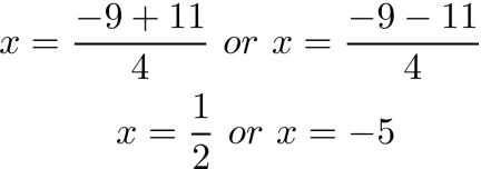
We will now plug in the values and determine x.

Discriminant
The discriminant of a quadratic equation is used to determine the type if the answer you would get if you solve the equation. THere are three types of answers that you can get when solving a quadratic equation.
A complex solution involves the use of an imaginary number. This happens when the square root number is negative, which is technically impossible. To deal with this in math the letter i is used instead of the negative sign below is an example.

The actual formula for calculating the discriminant is already in the quadratic formula. You simply calculate only the information under the square root. This is shown below.

IN our first example, we got two real solutions. We will now confirm this by calculating the discriminant.

Are answer is positive, which means that we can expect to calculate to real solutions for this particular problem.
Conclusion
The quadratic formula provides another way to solve a quadratic equation. This is probably the easiest method to learn as it is simply a matter of plugging numbers into the formula. This may explain why the quadratic formula is frequently the first method algebra students learn for solving quadratic equations.
The discriminant is a shortcut calculation that allows you to determine the quality of the solutions you would get if you solve the equation.

Matrices are a common tool used in algebra. They provide a way to deal with equations that have commonly held variables. In this post, we learn some of the basics of developing matrices.
From Equation to Matrix
Using a matrix involves making sure that the same variables and constants are all in the same column in the matrix. This will allow you to do any elimination or substitution you may want to do in the future. Below is an example


Above we have a system of equations to the left and an augmented matrix to the right. If you look at the first column in the matrix it has the same values as the x variables in the system of equations (2 & 3). This is repeated for the y variable (-1 & 3) and the constant (-3 & 6).
The number of variables that can be included in a matrix is unlimited. Generally, when learning algebra, you will commonly see 2 & 3 variable matrices. The example above is a 2 variable matrix below is a three-variable matrix.


If you look closely you can see there is nothing here new except the z variable with its own column in the matrix.
Row Operations
When a system of equations is in an augmented matrix we can perform calculations on the rows to achieve an answer. You can switch the order of rows as in the following.

You can multiply a row by a constant of your choice. Below we multiple all values in row 2 by 2. Notice the notation in the middle as it indicates the action performed.

You can also add rows together. In the example below row 1 and row 2, are summed to create a new row 1.

You can even multiply a row by a constant and then sum it with another row to make a new row. Below we multiply row 2 by 2 and then sum it with row 1 to make a new row 1.

The purpose of row operations is to provide a way to solve a system of equations in a matrix. In addition, writing out the matrices provides a way to track the work that was done. It is easy to get confused even the actual math is simple
Conclusion
System of equations can be difficult to solve. However, the use of matrices can reduce the computational load needed to solve them. You do need to be careful with how you modify the rows and columns and this is where the use of row operations can be beneficial.

Compound inequalities are two inequalities that are joined by the word “and” or the word “or”. Solving a compound inequality means finding all values that make the compound inequality true.
For compound inequalities join ed by the word “and” we look for solutions that are true for both inequalities. Fo compound inequalities joined by the word “or” we look for solutions that work for either inequality.
It is also possible to graph compound inequalities on a number line as well as indicate the final answer using interval notation. Below is a compound inequality with the line graph solution

Solving the answer is the same as a regular equation. Below is the number line for this answer.

The empty circle at -8 means that -8 is not part of the solution. This means all values less than -8 are acceptable answers. This is why the line moves from right to left. All values less than -8 until infinity are acceptable answers. Below is the interval notation.

The parentheses mean that the value next to it is not included as a solution. This corresponds to the empty circle over the -8 in the lin graph. If the value should be included such as with a less/greater than sign you would use a bracket.
Double Inequality
A double inequality is a more concise version of a compound inequality. The goal is to isolate the variable in the middle. Below is an example

This is not complex. We simply isolate x in the middle using appropriate steps. The number line and interval notation or as follows

This time there is a bracket next to -4 which means that -4 is also a potential solution. In addition, notice how the -4 has a filled circle on the number line. This is another indication that -4 is a solution.
Practical Application
You have signed up for internet access through your cell phone. Your bill is a flat $49.00 per month please $0.05 per minute for internet use. How many minutes can you use internet per month if you want to keep your bill somewhere between $54-$74 per month?
Below is the solution using a double inequality
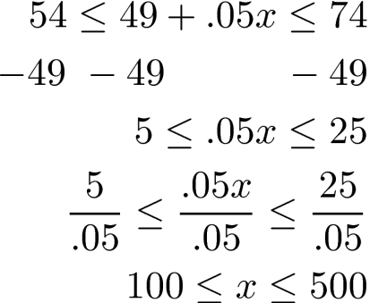
The answer indicates that you can spend anywhere from 100 to 500 minutes on the internet through your phone per month to stay within the budget. You can make the number line and develop the interval notation yourself.
Conclusion
Compound inequalities are useful for not only as an intellectual exercise. They can also be used to determine practical solutions that include more than one specific answer.

There are many examples in the world in which you want to know the quantity of several different items that make up a whole. When such a situation arise it is an example of mixture problem.
In this post, we will look at several examples of mixture problems. First, we need to look at the general equation for a mixture problem.
number * value = total value
The problems we will tackle will all involve some variation of the equation above. Below is our first example
Example 1
There are times when you want to figure out how many coins are needed to equal a certain dollar amount such as in the problem below
Tom has $6.04 of pennies and nickels. The number of nickels is 4 more and 6 times the number of pennies. How many nickels and pennies does Tom have?
To have success with this problem we need to convert the information into a table to see what we know. The table is below.
| Type | Number * | Value = | Total Value |
|---|---|---|---|
| Pennies | x | .01 | .01x |
| Nickels | 6x+4 | .05 | .05(6x+4) |
total 6.04
We can now solve our equation.

We know that there are 18.83 pennies. To determine the number of nickels we put 18.83 into x and get the following.
![]()
Almost 117 nickels
You can check if this works for yourself.
Example 2
For those of us who love to cook, mixture equations can be used for this as well below is an example.
Tom is mixing nuts and cranberries to make 20 pounds of trail mix. Nuts cost $8.00 per pound and cranberries cost $3.00 per pound. If Tom wants to his trail mix to cost $5.50 per pound how many pounds of raisins and cranberries should he use?
Our information is in the table below. What is new is subtracting the number of pounds from x. Doing so will help us to determine the number of pounds of cranberries.
| Type | Number of Pounds* | Price Per Pound = | Total Value |
|---|---|---|---|
| nuts | x | 8 | 8x |
| Cranberries | 20-x | 3 | 3(20-x) |
| Trail Mix | 20 | 5.5 | 20(5.50) |
We can now solve our equation with the information in the table above.

Once you solve for x you simply place this value into the equation. When you do this you see that we need ten pounds of nuts and berries to reach our target cost.
Conclusion
This post provided to practical examples of using algebra realistically. It is important to realize that understanding these basics concepts can be useful beyond the classroom.

This post will provide an explanation of how to solve equations that include fractions or decimals. The processes are similar in that both involve determining the least common denominator.
Solving Equations with Fractions
The key step to solving equations with fractions is to make sure that the denominators of all the fractions are the same. This can be done by finding the least common denominator. The least common denominator (LCD) is the smallest multiple of the denominators. For example, if we look at the multiples of 4 and 6 we see the following.

You can see clearly that the number 12 is the first multiple that 4 and 6 have in common. You can find the LCD by making factor trees but that is beyond the scope of this post. The primary reason we would need the LCD is when we are adding fractions in an equation. If we are multiplying we could simply multiply straight across.
Below is an equation that has fractions. We will find the LCD

Here is an explanation of each step
Solving Equations with Decimals
The process for solving equations with decimals is almost the same as for fractions. The LCD of all decimals is 100. Therefore, one common way to deal with decimals is to multiply all decimals by 100 and the continue to solve the equation.
The primary benefit of multiply by 100 is to remove the decimals because sometimes we make mistakes with where to place decimals. Below is an example of an equation with decimals.

Conclusion
Understand the process of solving equations with fractions or decimals is not to complicated. However, this information is much more valuable when dealing with more complex mathematical ideas.

In this post, we will look at several types of equations that you would encounter when learning algebra. Algebra is a foundational subject to know when conducting most quantitative research.
Equations
An equation is a statement that balances two expressions. Often equations include a variable or an unknown value. By solving for the unknown value you are able to balance the equation.
There are many different types of equations such as
(1) Linear equation
![]()
(2) Quadratic equation
![]()
(3) Polynomial equation
See number 1 or 2. The rule for polynomial equation is that the exponent must be positive
(4) Trigonometric equation
![]()
(5) Radical equation
![]()
(6) Exponential equation
![]()
This post will focus on linear equations.
Linear Equation
A linear equation is an equation that if it is graph will render a straight line. It is common to have to solve for the variable in a linear equation by isolating as in the example below.

There are also several terms related to equations and the include the following

Any value of x will work with an identity equation.

No value of x will work with the equation above.
Conclusion
This post provided an overview of the types of equations commonly encountered in algebra.

This post will provide insights into some basic algebraic concepts. Such information is actually useful for people who are doing research but may not have the foundational mathematical experience.
Multiple
A multiple is a product of n and a counting number of n. In the preceding sentence, we actually have two unknown values which are.
The n can be any value, while the counting number usually starts at 1 and continues by increasing by 1 each time until you want it to stop. This is how this would look if we used the term n, counting number, and multiple of n.
n * counting number = multiple of n
For example, if we say that n = 2 and the counting numbers are 1,2,3,4,5. We get the following multiples of 2.
![]()
You can see that the n never changes and remains constant as the value 2. The counting number starts at 1 and increases each time. Lastly, the multiple is the product of n and the counting number.
Let’s take one example from above
2 * 3 = 6
Here are some conclusions we can make from this simple equation
Divisibility Rules
There are also several divisibility rules in math. They can be used as shortcuts to determine if a number is divisible by another without having to do any calculation.
A number is divisible by
Factors
Factors are two or more numbers that when multiplied produce a number. For example

The numbers 7 and 6 are factors of 42. In other words, 7 and 6 are divisible by 42. A number that has only itself and one as factors is known as a prime number. Examples include 2, 3, 5, 7, 11, 13. A number that has many factors is called a composite number and includes such examples as 4, 8, 10, 12, 14.
An important concept in basic algebra is understanding how to find the prime numbers of a composite number. This is known as prime factorization and is done through the development of a factor tree. A factor tree breaks down a composite number into the various factors of it. These factors are further broken down into their factors until you reach the bottom of a tree that only contains prime numbers. Below is an example

You can see in the tree above that the prime factors of 12 are 2 and 3. If we take all of the prime factors and multiply them together we will get the answer 12.

Conclusion
Understanding these basic terms can only help someone who maybe jumped straight into statistics in grad school without have the prior thorough experience in basic algebra.


