Monthly Archives: March 2017

Ridge Regression in R

Advertisements

In this post, we will conduct an analysis using ridge regression. Ridge regression is a type of regularized regression. By applying a shrinkage penalty, we are able to reduce the coefficients of many variables almost to zero while still retaining them in the model. This allows us to develop models that have many more variables in them compared to models using the best subset or stepwise regression.

In the example used in this post, we will use the “SAheart” dataset from the “ElemStatLearn” package. We want to predict systolic blood pressure (sbp) using all of the other variables available as predictors. Below is some initial code that we need to begin.

library(ElemStatLearn);library(car);library(corrplot)
library(leaps);library(glmnet);library(caret)
data(SAheart)
str(SAheart)
## 'data.frame':    462 obs. of  10 variables:
##  $ sbp      : int  160 144 118 170 134 132 142 114 114 132 ...
##  $ tobacco  : num  12 0.01 0.08 7.5 13.6 6.2 4.05 4.08 0 0 ...
##  $ ldl      : num  5.73 4.41 3.48 6.41 3.5 6.47 3.38 4.59 3.83 5.8 ...
##  $ adiposity: num  23.1 28.6 32.3 38 27.8 ...
##  $ famhist  : Factor w/ 2 levels "Absent","Present": 2 1 2 2 2 2 1 2 2 2 ...
##  $ typea    : int  49 55 52 51 60 62 59 62 49 69 ...
##  $ obesity  : num  25.3 28.9 29.1 32 26 ...
##  $ alcohol  : num  97.2 2.06 3.81 24.26 57.34 ...
##  $ age      : int  52 63 46 58 49 45 38 58 29 53 ...
##  $ chd      : int  1 1 0 1 1 0 0 1 0 1 ...

A look at the object using the “str” function indicates that one variable “famhist” is a factor variable. The “glmnet” function that does the ridge regression analysis cannot handle factors so we need to convert this to a dummy variable. However, there are two things we need to do before this. First, we need to check the correlations to make sure there are no major issues with multicollinearity Second, we need to create our training and testing data sets. Below is the code for the correlation plot.

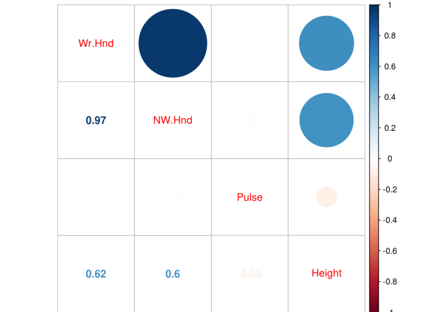
p.cor<-cor(SAheart[,-5])
corrplot.mixed(p.cor)

1

First we created a variable called “p.cor” the -5 in brackets means we removed the 5th column from the “SAheart” data set which is the factor variable “Famhist”. The correlation plot indicates that there is one strong relationship between adiposity and obesity. However, one common cut-off for collinearity is 0.8 and this value is 0.72 which is not a problem.

We will now create are training and testing sets and convert “famhist” to a dummy variable.

ind<-sample(2,nrow(SAheart),replace=T,prob = c(0.7,0.3))
train<-SAheart[ind==1,]
test<-SAheart[ind==2,]
train$famhist<-model.matrix( ~ famhist - 1, data=train ) #convert to dummy variable 
test$famhist<-model.matrix( ~ famhist - 1, data=test )

We are still not done preparing our data yet. “glmnet” cannot use data frames, instead, it can only use matrices. Therefore, we now need to convert our data frames to matrices. We have to create two matrices, one with all of the predictor variables and a second with the outcome variable of blood pressure. Below is the code

predictor_variables<-as.matrix(train[,2:10])
blood_pressure<-as.matrix(train$sbp)

We are now ready to create our model. We use the “glmnet” function and insert our two matrices. The family is set to Gaussian because “blood pressure” is a continuous variable. Alpha is set to 0 as this indicates ridge regression. Below is the code

ridge<-glmnet(predictor_variables,blood_pressure,family = 'gaussian',alpha = 0)

Now we need to look at the results using the “print” function. This function prints a lot of information as explained below.

  •  Df = number of variables including in the model (this is always the same number in a ridge model)
  •  %Dev = Percent of deviance explained. The higher the better
  • Lambda = The lambda used to attain the %Dev

When you use the “print” function for a ridge model it will print up to 100 different models. Fewer models are possible if the percent of deviance stops improving. 100 is the default stopping point. In the code below we have the “print” function. However, I have only printed the first 5 and last 5 models in order to save space.

print(ridge)
## 
## Call:  glmnet(x = predictor_variables, y = blood_pressure, family = "gaussian",      alpha = 0) 
## 
##        Df      %Dev    Lambda
##   [1,] 10 7.622e-37 7716.0000
##   [2,] 10 2.135e-03 7030.0000
##   [3,] 10 2.341e-03 6406.0000
##   [4,] 10 2.566e-03 5837.0000
##   [5,] 10 2.812e-03 5318.0000
................................
##  [95,] 10 1.690e-01    1.2290
##  [96,] 10 1.691e-01    1.1190
##  [97,] 10 1.692e-01    1.0200
##  [98,] 10 1.693e-01    0.9293
##  [99,] 10 1.693e-01    0.8468
## [100,] 10 1.694e-01    0.7716

The results from the “print” function are useful in setting the lambda for the “test” dataset. Based on the results we can set the lambda at 0.83 because this explains the highest amount of deviance at .20.

The plot below shows us lambda on the x-axis and the coefficients of the predictor variables on the y-axis. The numbers refer to the actual coefficient of a particular variable. Inside the plot, each number corresponds to a variable going from left to right in a data-frame/matrix using the “View” function. For example, 1 in the plot refers to “tobacco” 2 refers to “ldl” etc. Across the top of the plot is the number of variables used in the model. Remember this number never changes when doing ridge regression.

plot(ridge,xvar="lambda",label=T)

As you can see, as lambda increase the coefficient decrease in value. This is how ridge regression works yet no coefficient ever goes to absolute 0.

You can also look at the coefficient values at a specific lambda value. The values are unstandardized but they provide a useful insight when determining final model selection. In the code below the lambda is set to .83 and we use the “coef” function to do this

ridge.coef<-coef(ridge,s=.83,exact = T)
ridge.coef
## 11 x 1 sparse Matrix of class "dgCMatrix"
##                                   1
## (Intercept)            105.69379942
## tobacco                 -0.25990747
## ldl                     -0.13075557
## adiposity                0.29515034
## famhist.famhistAbsent    0.42532887
## famhist.famhistPresent  -0.40000846
## typea                   -0.01799031
## obesity                  0.29899976
## alcohol                  0.03648850
## age                      0.43555450
## chd                     -0.26539180

The second plot shows us the deviance explained on the x-axis and the coefficients of the predictor variables on the y-axis. Below is the code

plot(ridge,xvar='dev',label=T)

The two plots are completely opposite to each other. Increasing lambda cause a decrease in the coefficients while increasing the fraction of deviance explained leads to an increase in the coefficient. You can also see this when we used the “print” function. As lambda became smaller there was an increase in the deviance explained.

We now can begin testing our model on the test data set. We need to convert the test dataset to a matrix and then we will use the predict function while setting our lambda to .83 (remember a lambda of .83 explained the most of the deviance). Lastly, we will plot the results. Below is the code.

test.matrix<-as.matrix(test[,2:10])
ridge.y<-predict(ridge,newx = test.matrix,type = 'response',s=.83)
plot(ridge.y,test$sbp)

The last thing we need to do is calculated the mean squared error. By it’s self this number is useless. However, it provides a benchmark for comparing the current model with any other models you may develop. Below is the code

ridge.resid<-ridge.y-test$sbp
mean(ridge.resid^2)
## [1] 372.4431

Knowing this number, we can develop other models using other methods of analysis to try to reduce it as much as possible.

Regularized Linear Regression

Advertisements

Traditional linear regression has been a tried and true model for making predictions for decades. However, with the growth of Big Data and datasets with 100’s of variables problems have begun to arise. For example, using stepwise or best subset method with regression could take hours if not days to converge in even some of the best computers.

To deal with this problem, regularized regression has been developed to help to determine which features or variables to keep when developing models from large datasets with a huge number of variables. In this post, we will look at the following concepts

  • Definition of regularized regression
  • Ridge regression
  • Lasso regression
  • Elastic net regression

Regularization

Regularization involves the use of a shrinkage penalty in order to reduce the residual sum of squares (RSS). This is done by selecting a value for a tuning parameter called “lambda”. Tuning parameters are used in machine learning algorithms to control the behavior of the models that are developed.

The lambda is multiplied by the normalized coefficients of the model and added to the RSS. Below is an equation of what was just said

RSS + λ(normalized coefficients)

The benefits of regularization are at least three-fold. First, regularization is highly computationally efficient. Instead of fitting k-1 models when k is the number of variables available (for example, 50 variables would lead 49 models!), with regularization only one model is developed for each value of lambda you specify.

Second, regularization helps to deal with the bias-variance headache of model development. When small changes are made to data, such as switching from the training to testing data, there can be wild changes in the estimates. Regularization can often smooth this problem out substantially.

Finally, regularization can help to reduce or eliminate any multicollinearity in a model. As such, the benefits of using regularization make it clear that this should be considered when working with larger datasets.

Ridge Regression

Ridge regression involves the normalization of the squared weights or as shown in the equation below

RSS + λ(normalized coefficients^2)

This is also referred to as the L2-norm. As lambda increase in value, the coefficients in the model are shrunk towards 0 but never reach 0. This is how the error is shrunk. The higher the lambda the lower the value of the coefficients as they are reduced more and more thus reducing the RSS.

The benefit is that predictive accuracy is often increased. However, interpreting and communicating your results can become difficult because no variables are removed from the model. Instead, the variables are reduced near to zero. This can be especially tough if you have dozens of variables remaining in your model to try to explain.

Lasso

Lasso is short for “Least Absolute Shrinkage and Selection Operator”. This approach uses the L1-norm which is the sum of the absolute value of the coefficients or as shown in the equation below

RSS + λ(Σ|normalized coefficients|)

This shrinkage penalty will reduce a coefficient to 0 which is another way of saying that variables will be removed from the model. One problem is that highly correlated variables that need to be in your model may be removed when Lasso shrinks coefficients. This is one reason why ridge regression is still used.

Elastic Net

Elastic net is the best of ridge and Lasso without the weaknesses of either. It combines extracts variables like Lasso and Ridge does not while also group variables like Ridge does but Lasso does not.

This is done by including a second tuning parameter called “alpha”. If alpha is set to 0 it is the same as ridge regression and if alpha is set to 1 it is the same as lasso regression. If you are able to appreciate it below is the formula used for elastic net regression

(RSS + l[(1 – alpha)(S|normalized coefficients|2)/2 + alpha(S|normalized coefficients|)])/N)

As such when working with elastic net you have to set two different tuning parameters (alpha and lambda) in order to develop a model.

Conclusion

Regularized regression was developed as an answer to the growth in the size and number of variables in a data set today. Ridge, lasso an elastic net all provide solutions to converging over large datasets and selecting features.

Social Networks and Language Habits

Advertisements

In this post, we will look at how relationships that people have can play a role in how they communicate with those around them. Understanding this can help people to comprehend differences in communication style.

In sociolinguistics, social networks can refer to the pattern of informal relationships that people have and experience on a consistent basis. There are two dimensions that can be used to describe a person’s social network. These two terms are density and plexity.

Density

The density of a social network refers to how well people in your network know each other. In other words, density is how well your friends know each other. We all have friends, we have friends who know each other, and we have friends who do not know each other.

If many of your friends know each other then the density is high. If your friends do not know each other the density is low. An example of a high-density network would be the typical family. Everybody knows each other. An example of a low-density network would be employees at a large company. In such a situation it would not be hard to find a friend of a friend that you do not know.

Plexity

Plexity is a  measure of the various types of interactions that you are involved in with other people. Plexity can be uniplex, which involves one type of interaction with a person or multiplex, which involves many types of interactions with a person.

An example of a uniplex interaction may be a worker with their boss. They only interact at work. A multiplex interaction would again be with members of one’s family. When dealing with family interactions could include school, work, recreation, shopping, etc. In all these examples it is the same people interacting in a multitude of settings.

Language Use in Social Networks

A person’s speech almost always reflects the network that they belong too. If the group is homogeneous we will almost always speak the way everyone else does assuming we want to be a part of the group. For example, a group of local construction workers will more than likely use similar language patterns due to the homogeneous nature of the group while a group of ESL bankers would not as they come from many different countries.

When a person belongs to more than one social network they will almost always unconsciously change the way they communicate based on the context. For example, anybody who has moved away from home communicates differently where they live than when they communicate with family and friends back home. This is true even when moving from one place to another in the same province or state in your country.

Conclusion

The language that people employ is affected by the dynamics of the social network. We naturally will adjust our communication to accommodate who we are talking too.

Each Person Post One Discussion Forum in Moodle VIDEO

Advertisements

Using the Moodle forum option  of each person posts one discussion

Primary Tasks in Data Analysis

Advertisements

Performing a data analysis in the realm of data science is a difficult task due to the huge number of decisions that need to be made. For some people,  plotting the course to conduct an analysis is easy. However, for most of us, beginning a project leads to a sense of paralysis as we struggle to determine what to do.

In light of this challenge, there are at least 5 core task that you need to consider when preparing to analyze data. These five tasks are

  1. Developing  your question(s)
  2. Data exploration
  3. Developing a statistical model
  4. Interpreting the results
  5. Sharing the results

Developing Your Question(s)

You really cannot analyze data until you first determine what it is you want to know. It is tempting to just jump in and start looking for interesting stuff but you will not know if something you find is interesting unless it helps to answer your question(s).

There are several types of research questions. The point is you need to ask them in order to answer them.

Data Exploration

Data exploration allows you to determine if you can answer your questions with the data you have. In data science, the data is normally already collected by the time you are called upon to analyze it. As such, what you want to find may not be possible.

In addition, exploration of the data allows you to determine if there are any problems with the data set such as missing data, strange variables, and if necessary to develop a data dictionary so you know the characteristics of the variables.

Data exploration allows you to determine what kind of data wrangling needs to be done. This involves the preparation of the data for a more formal analysis when you develop your statistical models. This process takes up the majority of a data scientist time and is not easy at all.  Mastery of this in many ways means being a master of data science

Develop a Statistical Model

Your research questions and the data exploration process helps you to determine what kind of model to develop. The factors that can affect this is whether your data is supervised or unsupervised and whether you want to classify or predict numerical values.

This is probably the funniest part of data analysis and is much easier than having to wrangle with the data. Your goal is to determine if the model helps to answer your question(s)

Interpreting the Results

Once a model is developed it is time to explain what it means. Sometimes you can make a really cool model that nobody (including yourself) can explain. This is especially true of “black box” methods such as support vector machines and artificial neural networks. Models need to normally be explainable to non-technical stakeholders.

With interpretation, you are trying to determine “what does this answer mean to the stakeholders?”  For example, if you find that people who smoke are 5 times more likely to die before the age of 50 what are the implications of this? How can the stakeholders use this information to achieve their own goals? In other words, why should they care about what you found out?

Communication of Results

Now is the time to actually share the answer(s) to your question(s). How this is done varies but it can be written, verbal or both. Whatever the mode of communication it is necessary to consider the following

  • The audience or stakeholders
  • The actual answers to the questions
  • The benefits of knowing this

You must remember the stakeholders because this affects how you communicate. How you speak to business professionals would be different from academics. Next, you must share the answers to the questions. This can be done with charts, figures, illustrations etc. Data visualization is an expertise of its own. Lastly, you explain how this information is useful in a practical way.

Conclusion

The process shared here is one way to approach the analysis of data. Think of this as a framework from which to develop your own method of analysis.

Linear VS Quadratic Discriminant Analysis in R

Advertisements

In this post, we will look at linear discriminant analysis (LDA) and quadratic discriminant analysis (QDA). Discriminant analysis is used when the dependent variable is categorical. Another commonly used option is logistic regression but there are differences between logistic regression and discriminant analysis. Both LDA and QDA are used in situations in which there is a clear separation between the classes you want to predict. If the categories are fuzzier logistic regression is often the better choice.

For our example, we will use the “Mathlevel” dataset found in the “Ecdat” package. Our goal will be to predict the sex of a respondent based on SAT math score, major, foreign language proficiency, as well as the number of math, physic, and chemistry classes a respondent took. Below is some initial code to start our analysis.

library(MASS);library(Ecdat)
data("Mathlevel")

The first thing we need to do is clean up the data set. We have to remove any missing data in order to run our model. We will create a dataset called “math” that has the “Mathlevel” dataset but with the “NA”s removed use the “na.omit” function. After this, we need to set our seed for the purpose of reproducibility using the “set.seed” function. Lastly, we will split the data using the “sample” function using a 70/30 split. The training dataset will be called “math.train” and the testing dataset will be called “math.test”. Below is the code

math<-na.omit(Mathlevel)
set.seed(123)
math.ind<-sample(2,nrow(math),replace=T,prob = c(0.7,0.3))
math.train<-math[math.ind==1,]
math.test<-math[math.ind==2,]

Now we will make our model and it is called “lda.math” and it will include all available variables in the “math.train” dataset. Next, we will check the results by calling the model. Finally, we will examine the plot to see how our model is doing. Below is the code.

lda.math<-lda(sex~.,math.train)
lda.math
## Call:
## lda(sex ~ ., data = math.train)
## 
## Prior probabilities of groups:
##      male    female 
## 0.5986079 0.4013921 
## 
## Group means:
##        mathlevel.L mathlevel.Q mathlevel.C mathlevel^4 mathlevel^5
## male   -0.10767593  0.01141838 -0.05854724   0.2070778  0.05032544
## female -0.05571153  0.05360844 -0.08967303   0.2030860 -0.01072169
##        mathlevel^6      sat languageyes  majoreco  majoross   majorns
## male    -0.2214849 632.9457  0.07751938 0.3914729 0.1472868 0.1782946
## female  -0.2226767 613.6416  0.19653179 0.2601156 0.1907514 0.2485549
##          majorhum mathcourse physiccourse chemistcourse
## male   0.05426357   1.441860    0.7441860      1.046512
## female 0.07514451   1.421965    0.6531792      1.040462
## 
## Coefficients of linear discriminants:
##                       LD1
## mathlevel.L    1.38456344
## mathlevel.Q    0.24285832
## mathlevel.C   -0.53326543
## mathlevel^4    0.11292817
## mathlevel^5   -1.24162715
## mathlevel^6   -0.06374548
## sat           -0.01043648
## languageyes    1.50558721
## majoreco      -0.54528930
## majoross       0.61129797
## majorns        0.41574298
## majorhum       0.33469586
## mathcourse    -0.07973960
## physiccourse  -0.53174168
## chemistcourse  0.16124610
plot(lda.math,type='both')

Calling “lda.math” gives us the details of our model. It starts be indicating the prior probabilities of someone being male or female. Next is the means for each variable by sex. The last part is the coefficients of the linear discriminants. Each of these values is used to determine the probability that a particular example is male or female. This is similar to a regression equation.

The plot provides us with densities of the discriminant scores for males and then for females. The output indicates a problem. There is a great deal of overlap between male and females in the model. What this indicates is that there is a lot of misclassification going on as the two groups are not clearly separated. Furthermore, this means that logistic regression is probably a better choice for distinguishing between male and females. However, since this is for demonstrating purposes we will not worry about this.

We will now use the “predict” function on the training set data to see how well our model classifies the respondents by gender. We will then compare the prediction of the model with the actual classification. Below is the code.

math.lda.predict<-predict(lda.math)
math.train$lda<-math.lda.predict$class
table(math.train$lda,math.train$sex)
##         
##          male female
##   male    219    100
##   female   39     73
mean(math.train$lda==math.train$sex)
## [1] 0.6774942

As you can see, we have a lot of misclassification happening. A large amount of false negatives which is a lot of males being classified as female. The overall accuracy is only 59% which is not much better than chance.

We will now conduct the same analysis on the test data set. Below is the code.

lda.math.test<-predict(lda.math,math.test)
math.test$lda<-lda.math.test$class
table(math.test$lda,math.test$sex)
##         
##          male female
##   male     92     43
##   female   23     20
mean(math.test$lda==math.test$sex)
## [1] 0.6292135

As you can see the results are similar. To put it simply, our model is terrible. The main reason is that there is little distinction between males and females as shown in the plot. However, we can see if perhaps a quadratic discriminant analysis will do better

QDA allows for each class in the dependent variable to have its own covariance rather than a shared covariance as in LDA. This allows for quadratic terms in the development of the model. To complete a QDA we need to use the “qda” function from the “MASS” package. Below is the code for the training data set.

math.qda.fit<-qda(sex~.,math.train)
math.qda.predict<-predict(math.qda.fit)
math.train$qda<-math.qda.predict$class
table(math.train$qda,math.train$sex)
##         
##          male female
##   male    215     84
##   female   43     89
mean(math.train$qda==math.train$sex)
## [1] 0.7053364

You can see there is almost no difference. Below is the code for the test data.

math.qda.test<-predict(math.qda.fit,math.test)
math.test$qda<-math.qda.test$class
table(math.test$qda,math.test$sex)
##         
##          male female
##   male     91     43
##   female   24     20
mean(math.test$qda==math.test$sex)
## [1] 0.6235955

Still disappointing. However, in this post, we reviewed linear discriminant analysis as well as learned about the use of quadratic linear discriminant analysis. Both of these statistical tools are used for predicting categorical dependent variables. LDA assumes shared covariance in the dependent variable categories will QDA allows for each category in the dependent variable to have its own variance.

Sociolinguistic Insights into Female Communication

Advertisements

In general, women tend to prefer to use the most standard or prestige form of a language regardless of cultural background or geography. Linguists have proposed several potential reasons for this. This post will share some of the most common ideas on why women often used the standard form of their language.

Social Status

There is a belief among many linguists that women use the most prestigious forms of their language because they are more status-conscious than men. By using the standard version of their language a woman is able to claim a higher status.

The implication of this is that women have a lower status in society and try to elevate themselves through their use of language. However, this conclusion has been refuted as women who work outside the home use more of the standard form of their language than women who work in their home.

If the social status hypothesis was correct women who work at home, and thus have the lowest status, should use more of the standard form then women who work. Currently, this is not the case.

Women as Protector of Society’s Values

The women as protector of values view see social pressure as a constraint on how women communicate. Simply, women use more standard forms of their language than men because women are expected to behave better. It is thrust upon women to serve as an example for their community and especially for their children.

This answer is considered correct but depends highly on context. For example, this idea falls a part most frequently when women communicate with their children. The informal and intimate setting often leads to most women using the vernacular aspects of their language.

Women as Subordinate Group

A third suggestion is that women, who are often a subordinate group, use the more standard version of their language to show deference to those over them. In other words, women use the most polite forms of their language to avoid offending men.

However, this suggestion also fails because it equates politeness with the standard form of a language. People can be polite using vernacular and they can be rude using the most prestigious form of their language possible.

Vernacular as Masculine

A final common hypothesis on women’s use of standard forms is the perception that the use of the vernacular is masculine and tough. Women choose the standard form as a way of demonstrating behaviors traditionally associated with gender in their culture. Men, on the other hand, use vernacular forms to show traits that are traditionally associated with male behaviors.

The problem with this belief is the informal settings. As mentioned previously, women and men use more vernacular forms of their language in informal settings. As such, it seems that context is one of the strongest factors in how language is used and not necessarily gender.

Discrete-Point and Integrative Language Testing Methods

Advertisements

Within language testing, there has arisen over time at least two major viewpoints on assessment. Originally,  the view was that assessing language should look specific elements of a language or you could say that language assessment should look at discrete aspects of the language.

A reaction to this discrete methods came about with the idea that language is wholistic so testing should be integrative or address many aspects of language simultaneously. In this post, we will take a closer look at discrete and integrative language testing methods through providing examples of each along with a comparison.

Discrete-Point Testing

Discrete-point testing works on the assumption that language can be reduced to several discrete component “points” and that these “points” can be assessed. Examples of discrete-point test items in language testing include multiple choice, true/false, fill in the blank, and spelling.

What all of these example items have in common is that they usually isolate an aspect of the language from the broader context. For example, a simple spelling test is highly focused on the orthographic characteristics of the language. True/false can be used to assess knowledge of various grammar rules etc.

The primary criticism of discrete-point testing was its discreteness. Many believe that language is wholistic and that in the real world students will never have to deal with language in such an isolated way. This led to the development of integrative language testing methods.

Integrative Language Testing Methods

Integrative language testing is based on the unitary trait hypothesis, which states that language is indivisible. This is in complete contrast to discrete-point methods which supports dividing language into specific components.  Two common integrative language assessments include cloze test and dictation.

Cloze test involves taking an authentic reading passage and removing words from it. Which words remove depends on the test creator. Normally, it is every 6th or 7th word but it could be more or less or only the removal of key vocabulary. In addition, sometimes potential words are given to the student to select from or sometimes the list of words is not given to the student

The student’s job is to look at the context of the entire story to determine which words to write into the blank space.  This is an integrative experience as the students have to consider grammar, vocabulary, context, etc. to complete the assessment.

Dictation is simply writing down what was heard. This also requires the use of several language skills simultaneously in a realistic context.

Integrative language testing also has faced criticism. For example, discrete-point testing has always shown that people score differently in different language skills and this fact has been replicated in many studies. As such, the exclusive use of integrative language approaches is not supported by most TESOL scholars.

Conclusion

As with many other concepts in education, the best choice between discrete-point and integrative testing is a combination of both. The exclusive use of either will not allow the students to demonstrate mastery of the language.

Validating a Logistic Model in R

Advertisements

In this post, we are going to continue our analysis of the logistic regression model from the post on logistic regression in R. We need to rerun all of the code from the last post to be ready to continue. As such the code form the last post is all below

library(MASS);library(bestglm);library(reshape2);library(corrplot);
library(ggplot2);library(ROCR)
data(survey)
survey$Clap<-NULL
survey$W.Hnd<-NULL
survey$Fold<-NULL
survey$Exer<-NULL
survey$Smoke<-NULL
survey$M.I<-NULL
survey<-na.omit(survey)
pm<-melt(survey, id.var="Sex")
ggplot(pm,aes(Sex,value))+geom_boxplot()+facet_wrap(~variable,ncol = 3)

pc<-cor(survey[,2:5])
corrplot.mixed(pc)

set.seed(123) ind<-sample(2,nrow(survey),replace=T,prob = c(0.7,0.3)) train<-survey[ind==1,] test<-survey[ind==2,] fit<-glm(Sex~.,binomial,train) exp(coef(fit))

train$probs<-predict(fit, type = 'response')
train$predict<-rep('Female',123)
train$predict[train$probs>0.5]<-"Male"
table(train$predict,train$Sex)
mean(train$predict==train$Sex)
test$prob<-predict(fit,newdata = test, type = 'response')
test$predict<-rep('Female',46)
test$predict[test$prob>0.5]<-"Male"
table(test$predict,test$Sex)
mean(test$predict==test$Sex)

Model Validation

We will now do a K-fold cross validation in order to further see how our model is doing. We cannot use the factor variable “Sex” with the K-fold code so we need to create a dummy variable. First, we create a variable called “y” that has 123 spaces, which is the same size as the “train” dataset. Second, we fill “y” with 1 in every example that is coded “male” in the “Sex” variable.

In addition, we also need to create a new dataset and remove some variables from our prior analysis otherwise we will confuse the functions that we are going to use. We will remove “predict”, “Sex”, and “probs”

train$y<-rep(0,123)
train$y[train$Sex=="Male"]=1
my.cv<-train[,-8]
my.cv$Sex<-NULL
my.cv$probs<-NULL

We now can do our K-fold analysis. The code is complicated so you can trust it and double check on your own.

bestglm(Xy=my.cv,IC="CV",CVArgs = list(Method="HTF",K=10,REP=1),family = binomial)
## Morgan-Tatar search since family is non-gaussian.
## CV(K = 10, REP = 1)
## BICq equivalent for q in (6.66133814775094e-16, 0.0328567092272112)
## Best Model:
##                Estimate Std. Error   z value     Pr(>|z|)
## (Intercept) -45.2329733 7.80146036 -5.798014 6.710501e-09
## Height        0.2615027 0.04534919  5.766425 8.097067e-09

The results confirm what we alreaedy knew that only the “Height” variable is valuable in predicting Sex. We will now create our new model using only the recommendation of the kfold validation analysis. Then we check the new model against the train dataset and with the test dataset. The code below is a repeat of prior code but based on the cross-validation

reduce.fit<-glm(Sex~Height, family=binomial,train)
train$cv.probs<-predict(reduce.fit,type='response')
train$cv.predict<-rep('Female',123)
train$cv.predict[train$cv.probs>0.5]='Male'
table(train$cv.predict,train$Sex)
##         
##          Female Male
##   Female     61   11
##   Male        7   44
mean(train$cv.predict==train$Sex)
## [1] 0.8536585
test$cv.probs<-predict(reduce.fit,test,type = 'response')
test$cv.predict<-rep('Female',46)
test$cv.predict[test$cv.probs>0.5]='Male'
table(test$cv.predict,test$Sex)
##         
##          Female Male
##   Female     16    7
##   Male        1   22
mean(test$cv.predict==test$Sex)
## [1] 0.826087

The results are consistent for both the train and test dataset. We are now going to create the ROC curve. This will provide a visual and the AUC number to further help us to assess our model. However, a model is only good when it is compared to another model. Therefore, we will create a really bad model in order to compare it to the original model, and the cross validated model. We will first make a bad model and store the probabilities in the “test” dataset. The bad model will use “age” to predict “Sex” which doesn’t make any sense at all. Below is the code followed by the ROC curve of the bad model.

bad.fit<-glm(Sex~Age,family = binomial,test)
test$bad.probs<-predict(bad.fit,type='response')
pred.bad<-prediction(test$bad.probs,test$Sex)
perf.bad<-performance(pred.bad,'tpr','fpr')
plot(perf.bad,col=1)

The more of a diagonal the line is the worst it is. As we can see the bad model is really bad.

What we just did with the bad model we will now repeat for the full model and the cross-validated model.  As before, we need to store the prediction in a way that the ROCR package can use them. We will create a variable called “pred.full” to begin the process of graphing the original full model from the last blog post. Then we will use the “prediction” function. Next, we will create the “perf.full” variable to store the performance of the model. Notice, the arguments ‘tpr’ and ‘fpr’ for true positive rate and false positive rate. Lastly, we plot the results

pred.full<-prediction(test$prob,test$Sex)
perf.full<-performance(pred.full,'tpr','fpr')
plot(perf.full, col=2)

We repeat this process for the cross-validated model

pred.cv<-prediction(test$cv.probs,test$Sex)
perf.cv<-performance(pred.cv,'tpr','fpr')
plot(perf.cv,col=3)

Now let’s put all the different models on one plot

plot(perf.bad,col=1)
plot(perf.full, col=2, add=T)
plot(perf.cv,col=3,add=T)
legend(.7,.4,c("BAD","FULL","CV"), 1:3)

Finally, we can calculate the AUC for each model

auc.bad<-performance(pred.bad,'auc')
auc.bad@y.values
## [[1]]
## [1] 0.4766734
auc.full<-performance(pred.full,"auc")
auc.full@y.values
## [[1]]
## [1] 0.959432
auc.cv<-performance(pred.cv,'auc')
auc.cv@y.values
## [[1]]
## [1] 0.9107505

The higher the AUC the better. As such, the full model with all variables is superior to the cross-validated or bad model. This is despite the fact that there are many high correlations in the full model as well. Another point to consider is that the cross-validated model is simpler so this may be a reason to pick it over the full model. As such, the statistics provide support for choosing a model but they do not trump the ability of the research to pick based on factors beyond just numbers.

Logistic Regression in R

Advertisements

In this post, we will conduct a logistic regression analysis. Logistic regression is used when you want to predict a categorical dependent variable using continuous or categorical dependent variables. In our example, we want to predict Sex (male or female) when using several continuous variables from the “survey” dataset in the “MASS” package.

library(MASS);library(bestglm);library(reshape2);library(corrplot)
data(survey)
?MASS::survey #explains the variables in the study

The first thing we need to do is remove the independent factor variables from our dataset. The reason for this is that the function that we will use for the cross-validation does not accept factors. We will first use the “str” function to identify factor variables and then remove them from the dataset. We also need to remove in examples that are missing data so we use the “na.omit” function for this. Below is the code

survey$Clap<-NULL
survey$W.Hnd<-NULL
survey$Fold<-NULL
survey$Exer<-NULL
survey$Smoke<-NULL
survey$M.I<-NULL
survey<-na.omit(survey)

We now need to check for collinearity using the “corrplot.mixed” function form the “corrplot” package.

pc<-cor(survey[,2:5])
corrplot.mixed(pc)
corrplot.mixed(pc)

We have an extreme correlation between “We.Hnd” and “NW.Hnd” this makes sense because people’s hands are normally the same size. Since this blog post is a demonstration of logistic regression we will not worry about this too much.

We now need to divide our dataset into a train and a test set. We set the seed for. First, we need to make a variable that we call “ind” that is randomly assigned 70% of the number of rows of survey 1 and 30% 2. We then subset the “train” dataset by taking all rows that are 1’s based on the “ind” variable and we create the “test” dataset for all the rows that line up with 2 in the “ind” variable. This means our data split is 70% train and 30% test. Below is the code

set.seed(123)
ind<-sample(2,nrow(survey),replace=T,prob = c(0.7,0.3))
train<-survey[ind==1,]
test<-survey[ind==2,]

We now make our model. We use the “glm” function for logistic regression. We set the family argument to “binomial”. Next, we look at the results as well as the odds ratios.

fit<-glm(Sex~.,family=binomial,train)
summary(fit)
## 
## Call:
## glm(formula = Sex ~ ., family = binomial, data = train)
## 
## Deviance Residuals: 
##     Min       1Q   Median       3Q      Max  
## -1.9875  -0.5466  -0.1395   0.3834   3.4443  
## 
## Coefficients:
##              Estimate Std. Error z value Pr(>|z|)    
## (Intercept) -46.42175    8.74961  -5.306 1.12e-07 ***
## Wr.Hnd       -0.43499    0.66357  -0.656    0.512    
## NW.Hnd        1.05633    0.70034   1.508    0.131    
## Pulse        -0.02406    0.02356  -1.021    0.307    
## Height        0.21062    0.05208   4.044 5.26e-05 ***
## Age           0.00894    0.05368   0.167    0.868    
## ---
## Signif. codes:  0 '***' 0.001 '**' 0.01 '*' 0.05 '.' 0.1 ' ' 1
## 
## (Dispersion parameter for binomial family taken to be 1)
## 
##     Null deviance: 169.14  on 122  degrees of freedom
## Residual deviance:  81.15  on 117  degrees of freedom
## AIC: 93.15
## 
## Number of Fisher Scoring iterations: 6
exp(coef(fit))
##  (Intercept)       Wr.Hnd       NW.Hnd        Pulse       Height 
## 6.907034e-21 6.472741e-01 2.875803e+00 9.762315e-01 1.234447e+00 
##          Age 
## 1.008980e+00

The results indicate that only height is useful in predicting if someone is a male or female. The second piece of code shares the odds ratios. The odds ratio tell how a one unit increase in the independent variable leads to an increase in the odds of being male in our model. For example, for every one unit increase in height there is a 1.23 increase in the odds of a particular example being male.

We now need to see how well our model does on the train and test dataset. We first capture the probabilities and save them to the train dataset as “probs”. Next we create a “predict” variable and place the string “Female” in the same number of rows as are in the “train” dataset. Then we rewrite the “predict” variable by changing any example that has a probability above 0.5 as “Male”. Then we make a table of our results to see the number correct, false positives/negatives. Lastly, we calculate the accuracy rate. Below is the code.

train$probs<-predict(fit, type = 'response')
train$predict<-rep('Female',123)
train$predict[train$probs>0.5]<-"Male"
table(train$predict,train$Sex)
##         
##          Female Male
##   Female     61    7
##   Male        7   48
mean(train$predict==train$Sex)
## [1] 0.8861789

Despite the weaknesses of the model with so many insignificant variables it is surprisingly accurate at 88.6%. Let’s see how well we do on the “test” dataset.

test$prob<-predict(fit,newdata = test, type = 'response')
test$predict<-rep('Female',46)
test$predict[test$prob>0.5]<-"Male"
table(test$predict,test$Sex)
##         
##          Female Male
##   Female     17    3
##   Male        0   26
mean(test$predict==test$Sex)
## [1] 0.9347826

As you can see, we do even better on the test set with an accuracy of 93.4%. Our model is looking pretty good and height is an excellent predictor of sex which makes complete sense. However, in the next post we will use cross-validation and the ROC plot to further assess the quality of it.

Teaching Vocabulary to ESL Students

Advertisements

Language acquisition requires the acquisition of thousands of words for fluent communication. This is a daunting task for the most talented and eager student. Fortunately, there are some basic concepts to keep in mind when teaching students vocabulary. This post will share some suggestion and help students to develop their vocabulary in the target language.

Learn Vocabulary in Context

A common technique for teaching vocabulary in language classrooms is out of context memorization. Students are given a long and often boring list of words to memorize. There is little immediate use of these words and they are quickly forgotten after the quiz.

Instead, it is better to teach new words within a framework in which they will be used. For example, students learn business terms through role play at a bank or store rather than through a stack of index cards. The context of the bank connects the words to a real-world setting, which is critical for retention in the long-term memory.

Reduce Reliance on Bilingual Dictionaries

This may seem like a surprise, however, the proliferation of bilingual dictionaries provides the definition to a word but does not normally help with memorization and the future use of the word. If the goal is communication then bilingual dictionaries will slow a student’s ability to achieve mastery.

Children learn a language much faster due in part to the immense effort it takes to learn what new words mean without the easy answer of a dictionary. The effort leads to memorization which allows for the use of the language. This serves as a valuable lesson for adults who prefer the easy route of bilingual dictionaries.

Set Aside Class Time to Deal with Vocabulary

The teacher should have a systematic plan for helping students to develop relevant vocabulary. This can be done through activities as well as the teaching of context clues. Vocabulary development needs to be intentional, which means there must be a systematic plan for supporting students in this.

However, there are also times were unplanned vocabulary teaching can take place. For example, while the students are reading together they become puzzled over a word you thought they knew (this is common). When this happens a break with explanation can be helpful. This is especially true if you let the students work together without dictionaries to try and determining the meaning of the word.

Conclusion

Vocabulary is a necessary element of language learning. It would be nice to ignore this but normally this is impossible.  As such, teachers need to support students in their vocabulary development.

Probability,Odds, and Odds Ratio

Advertisements

In logistic regression, there are three terms that are used frequently but can be confusing if they are not thoroughly explained. These three terms are probability, odds, and odds ratio. In this post, we will look at these three terms and provide an explanation of them.

Probability

Probability is probably (no pun intended) the easiest of these three terms to understand. Probability is simply the likelihood that a certain event will happen.  To calculate the probability in the traditional sense you need to know the number of events and outcomes to find the probability.

Bayesian probability uses prior probabilities to develop a posterior probability based on new evidence. For example, at one point during Super Bowl LI the Atlanta Falcons had a 99.7% chance of winning. This was base don such factors as the number points they were ahead and the time remaining.  As these changed, so did the probability of them winning. yet the Patriots still found a way to win with less than a 1% chance

Bayesian probability was also used for predicting who would win the 2016 US presidential race. It is important to remember that probability is an expression of confidence and not a guarantee as we saw in both examples.

Odds

Odds are the expression of relative probabilities. Odds are calculated using the following equation

probability of the event ⁄ 1 – probability of the event

For example, at one point during Super Bowl LI the odds of the Atlanta Falcons winning were as follows

0.997 ⁄ 1 – 0.997 = 332

This can be interpreted as the odds being 332 to 1! This means that Atlanta was 332 times more likely to win the Super Bowl then loss the Super Bowl.

Odds are commonly used in gambling and this is probably (again no pun intended) where most of us have heard the term before. The odds is just an extension of probabilities and they are most commonly expressed as a fraction such as one in four, etc.

Odds Ratio

A ratio is the comparison of two numbers and indicates how many times one number is contained or contains another number. For example, a ration of boys to girls is 5 to 1 it means that there are five boys for every one girl.

By extension odds ratio is the comparison of two different odds. For example, if the odds of Team A making the playoffs is 45% and the odds of Team B making the playoffs is 35% the odds ratio is calculated as follows.

0.45 ⁄ 0.35 = 1.28

Team A is 1.28 more likely to make the playoffs then Team B.

The value of the odds and the odds ratio can sometimes be the same.  Below is the odds ratio of the Atlanta Falcons winning and the New Patriots winning Super Bowl LI

0.997⁄ 0.003 = 332

As such there is little difference between odds and odds ratio except that odds ratio is the ratio of two odds ratio. As you can tell, there is a lot of confusion about this for the average person. However, understanding these terms is critical to the application of logistic regression.