In this post, we will look at an example of regression trees. Regression trees use decision tree-like approach to develop prediction models involving numerical data. In our example, we will be trying to predict how many kids a person has based on several independent variables in the “PSID” data set in the “Ecdat” package.

Let’s begin by loading the necessary packages and data set. The code is below

library(Ecdat);library(rpart);library(rpart.plot)

library(RWeka)
data(PSID)
str(PSID)

## 'data.frame':    4856 obs. of  8 variables:
##  $ intnum  : int  4 4 4 4 5 6 6 7 7 7 ...
##  $ persnum : int  4 6 7 173 2 4 172 4 170 171 ...
##  $ age     : int  39 35 33 39 47 44 38 38 39 37 ...
##  $ educatn : int  12 12 12 10 9 12 16 9 12 11 ...
##  $ earnings: int  77250 12000 8000 15000 6500 6500 7000 5000 21000 0 ...
##  $ hours   : int  2940 2040 693 1904 1683 2024 1144 2080 2575 0 ...
##  $ kids    : int  2 2 1 2 5 2 3 4 3 5 ...
##  $ married : Factor w/ 7 levels "married","never married",..: 1 4 1 1 1 1 1 4 1 1 ...

summary(PSID)

##      intnum        persnum            age           educatn     
##  Min.   :   4   Min.   :  1.00   Min.   :30.00   Min.   : 0.00  
##  1st Qu.:1905   1st Qu.:  2.00   1st Qu.:34.00   1st Qu.:12.00  
##  Median :5464   Median :  4.00   Median :38.00   Median :12.00  
##  Mean   :4598   Mean   : 59.21   Mean   :38.46   Mean   :16.38  
##  3rd Qu.:6655   3rd Qu.:170.00   3rd Qu.:43.00   3rd Qu.:14.00  
##  Max.   :9306   Max.   :205.00   Max.   :50.00   Max.   :99.00  
##                                                  NA's   :1      
##     earnings          hours           kids                 married    
##  Min.   :     0   Min.   :   0   Min.   : 0.000   married      :3071  
##  1st Qu.:    85   1st Qu.:  32   1st Qu.: 1.000   never married: 681  
##  Median : 11000   Median :1517   Median : 2.000   widowed      :  90  
##  Mean   : 14245   Mean   :1235   Mean   : 4.481   divorced     : 645  
##  3rd Qu.: 22000   3rd Qu.:2000   3rd Qu.: 3.000   separated    : 317  
##  Max.   :240000   Max.   :5160   Max.   :99.000   NA/DF        :   9  
##                                                   no histories :  43

The variables “intnum” and “persnum” are for identification and are useless for our analysis. We will now explore our dataset with the following code.

hist(PSID$age)

hist(PSID$educatn)

hist(PSID$earnings)

hist(PSID$hours)

hist(PSID$kids)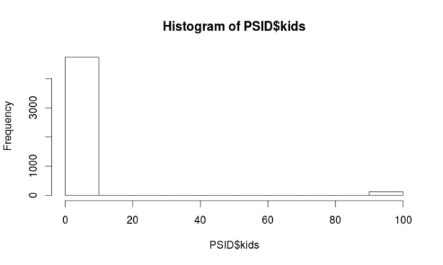

table(PSID$married)

## 
##       married never married       widowed      divorced     separated 
##          3071           681            90           645           317 
##         NA/DF  no histories 
##             9            43

Almost all of the variables are non-normal. However, this is not a problem when using regression trees. There are some major problems with the “kids” and “educatn” variables. Each of these variables has values at 98 and 99. When the data for this survey was collected 98 meant the respondent did not know the answer and a 99 means they did not want to say. Since both of these variables are numerical we have to do something with them so they do not ruin our analysis.

We are going to recode all values equal to or greater than 98 as 3 for the “kids” variable. The number 3 means they have 3 kids. This number was picked because it was the most common response for the other respondents. For the “educatn” variable all values equal to or greater than 98 are recoded as 12, which means that they completed 12th grade. Again this was the most frequent response. Below is the code.

PSID$kids[PSID$kids >= 98] <- 3
PSID$educatn[PSID$educatn >= 98] <- 12

Another peek at the histograms for these two variables and things look much better.

hist(PSID$kids)

hist(PSID$educatn)

Make Model and Visualization

Now that everything is cleaned up we now need to make our training and testing data sets as seen in the code below.

PSID_train<-PSID[1:3642,]
PSID_test<-PSID[3643:4856,]

We will now make our model and also create a visual of it. Our goal is to predict the number of children a person has based on their age, education, earnings, hours worked, marital status. Below is the code

#make model
PSID_Model<-rpart(kids~age+educatn+earnings+hours+married, PSID_train)
#make visualization
rpart.plot(PSID_Model, digits=3, fallen.leaves = TRUE,type = 3, extra=101)

The first split on the tree is by income. On the left, we have those who make more than 20k and on the right those who make less than 20k. On the left the next split is by marriage, those who are never married or not applicable have on average 0.74 kids. Those who are married, widowed, divorced, separated, or have no history have on average 1.72.

The left side of the tree is much more complicated and I will not explain all of it. The after making less than 20k the next split is by marriage. Those who are married, widowed, divorced, separated, or no history with less than 13.5 years of education have 2.46 on average.

Make Prediction Model and Conduct Evaluation

Our next task is to make the prediction model. We will do this with the following code

PSID_pred<-predict(PSID_Model, PSID_test)

We will now evaluate the model. We will do this three different ways. The first involves looking at the summary statistics of the prediction model and the testing data. The numbers should be about the same. After that, we will calculate the correlation between the prediction model and the testing data. Lastly, we will use a technique called the mean absolute error. Below is the code for the summary statistics and correlation.

summary(PSID_pred)

##    Min. 1st Qu.  Median    Mean 3rd Qu.    Max. 
##   0.735   2.041   2.463   2.226   2.463   2.699

summary(PSID_test$kids)

##    Min. 1st Qu.  Median    Mean 3rd Qu.    Max. 
##   0.000   2.000   2.000   2.494   3.000  10.000

cor(PSID_pred, PSID_test$kids)

## [1] 0.308116

Looking at the summary stats our model has a hard time predicting extreme values because the max value of the two models are far apart. However, how often do people have ten kids? As such, this is not a major concern.

A look at the correlation finds that it is pretty low (0.30) this means that the two models have little in common and this means we need to make some changes. The mean absolute error is a measure of the difference between the predicted and actual values in a model. We need to make a function first before we analyze our model.

MAE<-function(actual, predicted){
        mean(abs(actual-predicted))
}

We now assess the model with the code below

MAE(PSID_pred, PSID_test$kids)

## [1] 1.134968

The results indicate that on average the difference between our model’s prediction of the number of kids and the actual number of kids was 1.13 on a scale of 0 – 10. That’s a lot of error. However, we need to compare this number to how well the mean does to give us a benchmark. The code is below.

ave_kids<-mean(PSID_train$kids)
MAE(ave_kids, PSID_test$kids)

## [1] 1.178909

Model Tree

Our model with a score of 1.13 is slightly better than using the mean which is 1.17. We will try to improve our model by switching from a regression tree to a model tree which uses a slightly different approach for prediction. In a model tree each node in the tree ends in a linear regression model. Below is the code.

PSIDM5<- M5P(kids~age+educatn+earnings+hours+married, PSID_train)
PSIDM5

## M5 pruned model tree:
## (using smoothed linear models)
## 
## earnings <= 20754 : 
## |   earnings <= 2272 : 
## |   |   educatn <= 12.5 : LM1 (702/111.555%) ## |   |   educatn >  12.5 : LM2 (283/92%)
## |   earnings >  2272 : LM3 (1509/88.566%)
## earnings >  20754 : LM4 (1147/82.329%)
## 
## LM num: 1
## kids = 
##  0.0385 * age 
##  + 0.0308 * educatn 
##  - 0 * earnings 
##  - 0 * hours 
##  + 0.0187 * married=married,divorced,widowed,separated,no histories 
##  + 0.2986 * married=divorced,widowed,separated,no histories 
##  + 0.0082 * married=widowed,separated,no histories 
##  + 0.0017 * married=separated,no histories 
##  + 0.7181
## 
## LM num: 2
## kids = 
##  0.002 * age 
##  - 0.0028 * educatn 
##  + 0.0002 * earnings 
##  - 0 * hours 
##  + 0.7854 * married=married,divorced,widowed,separated,no histories 
##  - 0.3437 * married=divorced,widowed,separated,no histories 
##  + 0.0154 * married=widowed,separated,no histories 
##  + 0.0017 * married=separated,no histories 
##  + 1.4075
## 
## LM num: 3
## kids = 
##  0.0305 * age 
##  - 0.1362 * educatn 
##  - 0 * earnings 
##  - 0 * hours 
##  + 0.9028 * married=married,divorced,widowed,separated,no histories 
##  + 0.2151 * married=widowed,separated,no histories 
##  + 0.0017 * married=separated,no histories 
##  + 2.0218
## 
## LM num: 4
## kids = 
##  0.0393 * age 
##  - 0.0658 * educatn 
##  - 0 * earnings 
##  - 0 * hours 
##  + 0.8845 * married=married,divorced,widowed,separated,no histories 
##  + 0.3666 * married=widowed,separated,no histories 
##  + 0.0037 * married=separated,no histories 
##  + 0.4712
## 
## Number of Rules : 4

It would take too much time to explain everything. You can read part of this model as follows earnings greater than 20754 use linear model 4earnings less than 20754 and less than 2272 and less than 12.5 years of education use linear model 1 earnings less than 20754 and less than 2272 and greater than 12.5 years of education use linear model 2 earnings less than 20754 and greater than 2272 linear model 3 The print out then shows each of the linear model. Lastly, we will evaluate our model tree with the following code

PSIDM5_Pred<-predict(PSIDM5, PSID_test)
summary(PSIDM5_Pred)

##    Min. 1st Qu.  Median    Mean 3rd Qu.    Max. 
##  0.3654  2.0490  2.3400  2.3370  2.6860  4.4220

cor(PSIDM5_Pred, PSID_test$kids)

## [1] 0.3486492

MAE(PSID_test$kids, PSIDM5_Pred)

## [1] 1.088617

This model is slightly better. For example, it is better at predict extreme values at 4.4 compare to 2.69 for the regression tree model. The correlation is 0.34 which is better than 0.30 for the regression tree model. Lastly. the mean absolute error shows a slight improve to 1.08 compared to 1.13 in the regression tree model

Conclusion

This provide examples of the use of regression trees and model trees. Both of these models make prediction a key component of their analysis.