Decision trees are useful for splitting data based into smaller distinct groups based on criteria you establish. This post will attempt to explain how to develop decision trees in R.

We are going to use the ‘College’ dataset found in the “ISLR” package. Once you load the package you need to split the data into a training and testing set as shown in the code below. We want to divide the data based on education level, age, and income

library(ISLR); library(ggplot2); library(caret)
data("College")
inTrain<-createDataPartition(y=College$education, 
 p=0.7, list=FALSE)
trainingset <- College[inTrain, ]
testingset <- College[-inTrain, ]

Visualize the Data

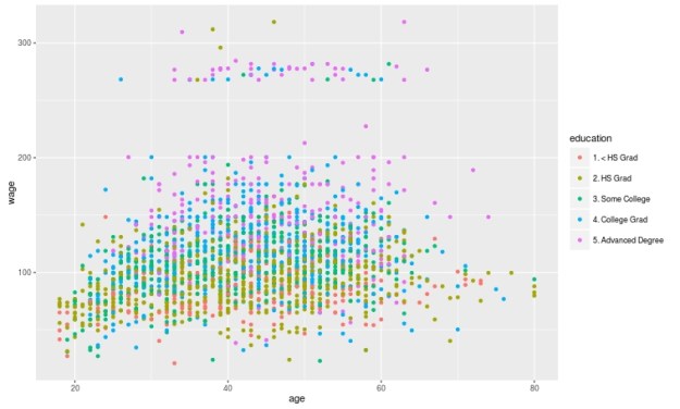
We will now make a plot of the data based on education as the groups and age and wage as the x and y variable. Below is the code followed by the plot. Please note that education is divided into 5 groups as indicated in the chart.

qplot(age, wage, colour=education, data=trainingset)

Create the Model

We are now going to develop the model for the decision tree. We will use age and wage to predict education as shown in the code below.

TreeModel<-train(education~age+income, method='rpart', data=trainingset)

Create Visual of the Model

We now need to create a visual of the model. This involves installing the package called ‘rattle’. You can install ‘rattle’ separately yourself. After doing this below is the code for the tree model followed by the diagram.

fancyRpartPlot(TreeModel$finalModel)

Here is what the chart means

1. At the top is node 1 which is called ‘HS Grad” the decimals underneath is the percentage of the data that falls within the “HS Grad” category. As the highest node, everything is classified as “HS grad” until we begin to apply our criteria.
2. Underneath nod 1 is a decision about wage. If a person makes less than 112 you go to the left if they make more you go to the right.
3. Nod 2 indicates the percentage of the sample that was classified as HS grade regardless of education. 14% of those with less than a HS diploma were classified as a HS Grade based on wage. 43% of those with a HS diploma were classified as a HS grade based on income. The percentage underneath the decimals indicates the total amount of the sample placed in the HS grad category. Which was 57%.
4. This process is repeated for each node until the data is divided as much as possible.

Predict

You can predict individual values in the dataset by using the ‘predict’ function with the test data as shown in the code below.

predict(TreeModel, newdata = testingset)

Conclusion

Prediction Trees are a unique feature in data analysis for determining how well data can be divided into subsets. It also provides a visual of how to move through data sequentially based on characteristics in the data.